How to perform dimensionality reduction on a mesh?#
Goal: get a lower-dimension representation of a mesh that can be fed to a regression model.
Hypotheses:
vertices are in one-to-one correspondence
Additional requirements:
pipeline should be invertible
pipeline must be compatible with
sklearn
[1]:
from pathlib import Path

import numpy as np
import pyvista as pv
from matplotlib import pyplot as plt
from sklearn.decomposition import PCA
from sklearn.preprocessing import FunctionTransformer, StandardScaler

import polpo.preprocessing.dict as ppdict
from polpo.plot.pyvista import RegisteredMeshesGifPlotter
from polpo.preprocessing import NestingSwapper
from polpo.preprocessing.load.pregnancy.jacobs import MeshLoader
from polpo.preprocessing.mesh.registration import RigidAlignment
from polpo.sklearn.adapter import AdapterPipeline
from polpo.sklearn.mesh import BiMeshesToVertices
from polpo.sklearn.np import BiFlattenButFirst
[KeOps] Warning : cuda was detected, but driver API could not be initialized. Switching to cpu only.
[2]:
STATIC_VIZ = True

if STATIC_VIZ:
    pv.set_jupyter_backend("static")
Loading meshes#
[3]:
subject_id = "01"

file_finder = MeshLoader(
    subject_subset=[subject_id],
    struct_subset=["L_Hipp"],
    as_mesh=True,
)

prep_pipe = RigidAlignment(max_iterations=500)

pipe = (
    file_finder
    + ppdict.ExtractUniqueKey(nested=True)
    + prep_pipe
    + ppdict.DictToValuesList()
)


meshes = pipe()
Create, fit and apply pipeline#
[4]:
pca = PCA(n_components=4)

objs2y = AdapterPipeline(
    steps=[
        BiMeshesToVertices(index=0),
        FunctionTransformer(func=np.stack),
        BiFlattenButFirst(),
        StandardScaler(with_std=False),
        pca,
    ],
)

objs2y
[4]:
AdapterPipeline(steps=[('step_0', BiMeshesToVertices()),
                       ('step_1',
                        FunctionTransformer(func=<function stack at 0x78a5facbf3f0>)),
                       ('step_2', BiFlattenButFirst()),
                       ('step_3', StandardScaler(with_std=False)),
                       ('step_4', PCA(n_components=4))])
In a Jupyter environment, please rerun this cell to show the HTML representation or trust the notebook. On GitHub, the HTML representation is unable to render, please try loading this page with nbviewer.org.
Parameters
| steps | [('step_0', ...), ('step_1', ...), ...] |
Parameters
| index | 0 |
Parameters
| func | <function sta...x78a5facbf3f0> | |
| inverse_func | None | |
| validate | False | |
| accept_sparse | False | |
| check_inverse | True | |
| feature_names_out | None | |
| kw_args | None | |
| inv_kw_args | None |
Parameters
Parameters
| copy | True | |
| with_mean | True | |
| with_std | False |
Parameters
| n_components | 4 | |
| copy | True | |
| whiten | False | |
| svd_solver | 'auto' | |
| tol | 0.0 | |
| iterated_power | 'auto' | |
| n_oversamples | 10 | |
| power_iteration_normalizer | 'auto' | |
| random_state | None |
[5]:
objs2y.fit(meshes);
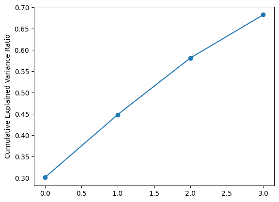
Let’s look at the explained variance ratio.
[6]:
plt.plot(np.cumsum(pca.explained_variance_ratio_), marker="o")

plt.ylabel("Cumulative Explained Variance Ratio");
Visualize changes along the PCA axes#
This is how the hippocampus changes when we move along the PCA axes.
[7]:
comps = objs2y.transform(meshes)

mean_comps = comps.mean(axis=0)

rec_meshes = []
for comp_index in range(4):
    sel_comps = comps[:, comp_index]

    min_sel_comp, max_sel_comp = np.min(sel_comps), np.max(sel_comps)

    var_comp = np.linspace(min_sel_comp, max_sel_comp, num=10)

    X = np.broadcast_to(mean_comps, (len(var_comp), comps.shape[1])).copy()
    X[:, comp_index] = var_comp

    rec_meshes.append(objs2y.inverse_transform(X))

rec_meshes = NestingSwapper()(rec_meshes)
[8]:
outputs_dir = Path("_images")
outputs_dir.mkdir(exist_ok=True)

gif_name = outputs_dir / "pca.gif"

pl = RegisteredMeshesGifPlotter(
    shape=(2, 2),
    gif_name=gif_name.as_posix(),
    fps=3,
    border=False,
    off_screen=True,
    notebook=False,
    subtitle=True,
)

pl.add_meshes(rec_meshes)
pl.close()

pl.show()
[8]: