Notebook source code: notebooks/05_explore_diffeomorphisms_of_space.ipynb
Explore Diffeomorphisms of Space#
Setup & Imports#
In [2]:
import setup
setup.main()
%load_ext autoreload
%autoreload 2
Working directory: /Users/facosta/Desktop/code/neurometry/neurometry/neuralwarp
Directory added to path: /Users/facosta/Desktop/code/neurometry/neurometry
Directory added to path: /Users/facosta/Desktop/code/neurometry/neurometry/neuralwarp
['/Users/facosta/Desktop/code/neurometry/neurometry/neuralwarp', '/Users/facosta/miniconda3/envs/neurometry/lib/python38.zip', '/Users/facosta/miniconda3/envs/neurometry/lib/python3.8', '/Users/facosta/miniconda3/envs/neurometry/lib/python3.8/lib-dynload', '', '/Users/facosta/miniconda3/envs/neurometry/lib/python3.8/site-packages', '/Users/facosta/Desktop/code/neurometry', '/Users/facosta/Desktop/code/neurometry/neurometry', '/Users/facosta/Desktop/code/neurometry/neurometry/neuralwarp']
Imports#
In [3]:
import pyLDDMM
from pyLDDMM.utils.visualization import loadimg, saveimg, save_animation, plot_warpgrid
import matplotlib.pyplot as plt
import numpy as np
from IPython.display import HTML
from matplotlib.animation import FuncAnimation
import torch
import os
os.environ["GEOMSTATS_BACKEND"] = "pytorch"
import geomstats.backend as gs
from geomstats.geometry.pullback_metric import PullbackMetric
INFO: Using pytorch backend
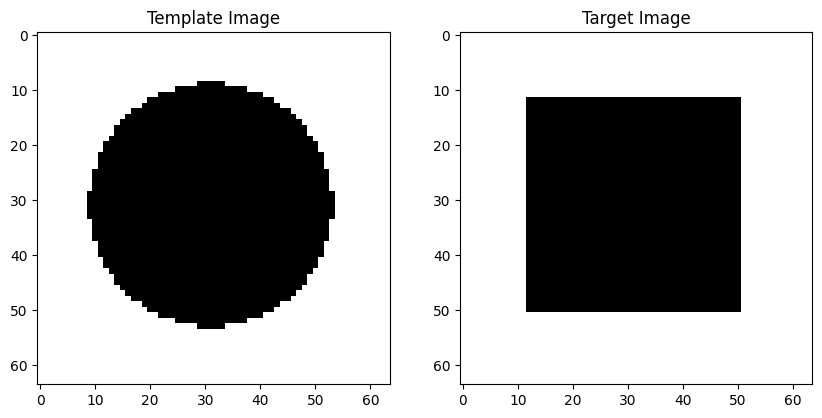
Examples: Circle to Square#
In [4]:
i0 = loadimg("./example_images/circle.png")
i1 = loadimg("./example_images/square.png")
fig = plt.figure(figsize=(10, 5))
ax1 = fig.add_subplot(121)
ax1.imshow(i0, cmap="gray")
ax1.set_title("Template Image")
ax2 = fig.add_subplot(122)
ax2.imshow(i1, cmap="gray")
ax2.set_title("Target Image");
Algorithm Inputs:#
\(I_0\): image, ndarray of dimension \(H \times W \times n\)
\(I_1\): image, ndarray of dimension \(H \times W \times n\)
\(T\): int, simulated discrete time steps
\(K\): int, maximum iterations
\(\sigma\): float, sigma for \(L_2\) loss. lower values strengthen the \(L_2\) loss
\(\alpha\): float, smoothness regularization. Higher values regularize stronger
\(\gamma\): float, norm penalty. Positive value to ensure injectivity of the regularizer
\(\epsilon\): float, learning rate
Algorithm Outputs:#
\(\phi_0\): forward flow
\(\phi_1\): backward flow
\(J_0\): time-series images generated by forward-pushing \(I_0\) using forward flow
\(J_1\): time-series images generated by pulling-back \(I_1\) using backward flow
\(\text{length}\): length of path on the manifold
\(v\): final velocity field
\(\text{energies}\):
\(\text{im}\): \(\text{im} = J_0[-1]\)
In [5]:
lddmm = pyLDDMM.LDDMM2D()
im, v, energies, length, Phi0, Phi1, J0, J1 = lddmm.register(
i0, i1, sigma=0.05, alpha=1, epsilon=0.0001, K=50
)
iteration 0, energy 110400.00, thereof 0.00 regularization and 110400.00 intensity difference
iteration 1, energy 31376.69, thereof 56.71 regularization and 31319.99 intensity difference
iteration 2, energy 12797.85, thereof 68.09 regularization and 12729.77 intensity difference
iteration 3, energy 8087.11, thereof 73.68 regularization and 8013.43 intensity difference
iteration 4, energy 5748.45, thereof 77.48 regularization and 5670.97 intensity difference
iteration 5, energy 4167.99, thereof 79.65 regularization and 4088.34 intensity difference
iteration 6, energy 3341.06, thereof 81.71 regularization and 3259.35 intensity difference
iteration 7, energy 3302.86, thereof 82.79 regularization and 3220.07 intensity difference
iteration 8, energy 3206.30, thereof 84.61 regularization and 3121.69 intensity difference
iteration 9, energy 3263.73, thereof 85.24 regularization and 3178.50 intensity difference
iteration 10, energy 3093.66, thereof 86.96 regularization and 3006.69 intensity difference
iteration 11, energy 3088.58, thereof 87.38 regularization and 3001.20 intensity difference
iteration 12, energy 2909.72, thereof 89.07 regularization and 2820.65 intensity difference
iteration 13, energy 2882.24, thereof 89.41 regularization and 2792.83 intensity difference
iteration 14, energy 2341.25, thereof 91.07 regularization and 2250.18 intensity difference
iteration 15, energy 2642.59, thereof 91.37 regularization and 2551.22 intensity difference
iteration 16, energy 2000.54, thereof 92.95 regularization and 1907.58 intensity difference
iteration 17, energy 2275.22, thereof 93.24 regularization and 2181.99 intensity difference
iteration 18, energy 1803.73, thereof 94.73 regularization and 1709.00 intensity difference
iteration 19, energy 2022.94, thereof 95.03 regularization and 1927.91 intensity difference
iteration 20, energy 1643.14, thereof 96.41 regularization and 1546.72 intensity difference
iteration 21, energy 1851.62, thereof 96.66 regularization and 1754.96 intensity difference
iteration 22, energy 1573.71, thereof 97.93 regularization and 1475.77 intensity difference
iteration 23, energy 1737.14, thereof 98.32 regularization and 1638.82 intensity difference
iteration 24, energy 1508.85, thereof 99.55 regularization and 1409.30 intensity difference
iteration 25, energy 1652.01, thereof 99.97 regularization and 1552.04 intensity difference
iteration 26, energy 1453.80, thereof 101.19 regularization and 1352.60 intensity difference
iteration 27, energy 1581.09, thereof 101.62 regularization and 1479.48 intensity difference
iteration 28, energy 1407.52, thereof 102.81 regularization and 1304.71 intensity difference
iteration 29, energy 1574.88, thereof 103.23 regularization and 1471.65 intensity difference
iteration 30, energy 1261.04, thereof 104.66 regularization and 1156.38 intensity difference
iteration 31, energy 1478.42, thereof 104.77 regularization and 1373.65 intensity difference
iteration 32, energy 1274.33, thereof 106.02 regularization and 1168.31 intensity difference
iteration 33, energy 1411.64, thereof 106.34 regularization and 1305.30 intensity difference
iteration 34, energy 1271.60, thereof 107.45 regularization and 1164.15 intensity difference
iteration 35, energy 1367.43, thereof 107.86 regularization and 1259.57 intensity difference
iteration 36, energy 1259.58, thereof 108.90 regularization and 1150.68 intensity difference
iteration 37, energy 1335.03, thereof 109.33 regularization and 1225.70 intensity difference
iteration 38, energy 1243.86, thereof 110.32 regularization and 1133.54 intensity difference
iteration 39, energy 1415.82, thereof 110.74 regularization and 1305.07 intensity difference
iteration 40, energy 1103.52, thereof 112.05 regularization and 991.47 intensity difference
iteration 41, energy 1306.41, thereof 112.13 regularization and 1194.28 intensity difference
iteration 42, energy 1133.39, thereof 113.22 regularization and 1020.16 intensity difference
iteration 43, energy 1244.86, thereof 113.54 regularization and 1131.32 intensity difference
iteration 44, energy 1147.82, thereof 114.45 regularization and 1033.38 intensity difference
iteration 45, energy 1210.97, thereof 114.87 regularization and 1096.10 intensity difference
iteration 46, energy 1151.12, thereof 115.69 regularization and 1035.43 intensity difference
iteration 47, energy 1191.13, thereof 116.16 regularization and 1074.97 intensity difference
iteration 48, energy 1149.42, thereof 116.92 regularization and 1032.51 intensity difference
iteration 49, energy 1300.43, thereof 117.39 regularization and 1183.04 intensity difference
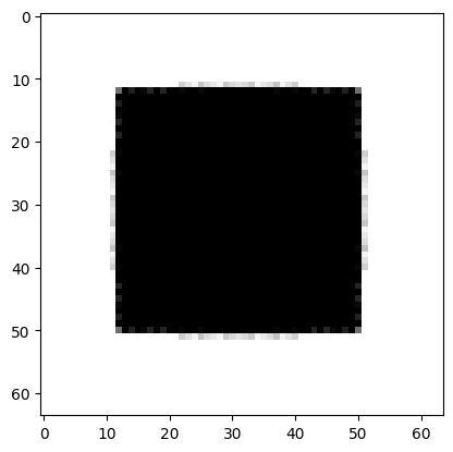
In [6]:
plt.imshow(im, cmap="gray");
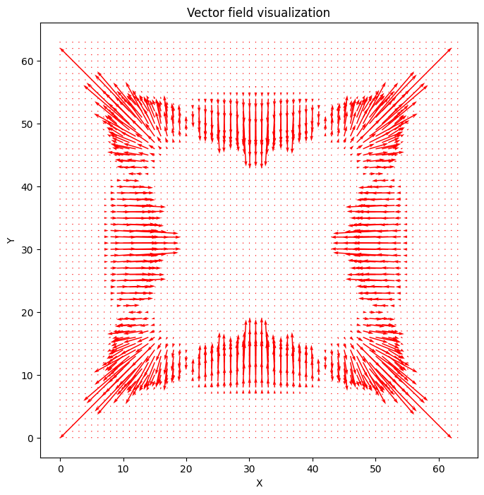
Visualize velocity vector field over time#
In [9]:
time_points = v.shape[0]
num_rows = v.shape[1]
num_columns = v.shape[2]
# Create a grid of points
x = np.linspace(0, num_columns - 1, num_columns)
y = np.linspace(0, num_rows - 1, num_rows)
X, Y = np.meshgrid(x, y)
fig, ax = plt.subplots(figsize=(8, 8))
# Create a quiver plot for the initial vector field
Q = ax.quiver(X, Y, v[0, :, :, 0], v[0, :, :, 1], color="red")
ax.set_title("Vector field visualization")
ax.set_xlabel("X")
ax.set_ylabel("Y")
# Update function for the animation
def update(num):
U = v[num, :, :, 0]
V = v[num, :, :, 1]
# Update the data for the quiver plot
Q.set_UVC(U, V)
return (Q,)
# Create the animation
ani = FuncAnimation(fig, update, frames=range(time_points), blit=True)
HTML(ani.to_jshtml());
INFO: Animation.save using <class 'matplotlib.animation.HTMLWriter'>
Out [9]:
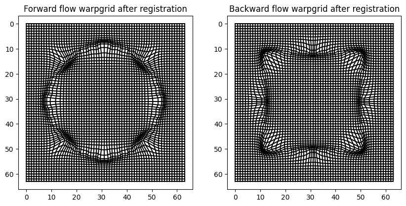
Visualize grid distortion#
In [7]:
fig = plt.figure(figsize=(10, 5))
ax0 = fig.add_subplot(121)
ax0 = plot_warpgrid(Phi0[-1], interval=1, show_axis=True)
ax0.set_title("Forward flow warpgrid after registration")
ax1 = fig.add_subplot(122)
ax1 = plot_warpgrid(Phi1[0], interval=1, show_axis=True)
ax1.set_title("Backward flow warpgrid after registration");
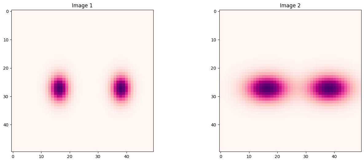
Examples: Distorted Gaussians#
In [26]:
from scipy.stats import multivariate_normal
def create_gaussian_image(width, height, resolution, x_variance, y_variance, distance):
x = np.linspace(0, width - 1, int(width / resolution))
y = np.linspace(0, height - 1, int(height / resolution))
x, y = np.meshgrid(x, y)
pos = np.dstack((x, y))
mu1 = np.array([width / 2 - distance / 2, height / 2])
cov1 = np.array([[x_variance, 0], [0, y_variance]]) # covariance matrix
rv1 = multivariate_normal(mu1, cov1)
mu2 = np.array([width / 2 + distance / 2, height / 2])
cov2 = np.array([[x_variance, 0], [0, y_variance]]) # covariance matrix
rv2 = multivariate_normal(mu2, cov2)
intensity_values1 = rv1.pdf(pos)
intensity_values2 = rv2.pdf(pos)
intensity_values = intensity_values1 + intensity_values2
intensity_values = intensity_values / np.sum(intensity_values)
return intensity_values
def create_uniform_image(width, height, resolution):
x = np.linspace(-1, 1, int(width / resolution))
y = np.linspace(-1, 1, int(height / resolution))
x, y = np.meshgrid(x, y)
# Calculate intensity values based on distance from center
intensity_values = np.ones_like(x)
intensity_values = intensity_values / np.sum(intensity_values)
return intensity_values
In [27]:
image1 = create_gaussian_image(
width=10, height=10, resolution=0.2, x_variance=0.2, y_variance=0.4, distance=4
)
image2 = create_gaussian_image(
width=10, height=10, resolution=0.2, x_variance=1, y_variance=0.4, distance=4
)
# image2 = create_uniform_image(width=5,height=5,resolution=0.1)
In [28]:
# Create a figure with two subplots side by side
fig, axs = plt.subplots(1, 2, figsize=(16, 6))
# Plot the first image on the first subplot
axs[0].imshow(image1, cmap="RdPu")
axs[0].set_title("Image 1")
# Plot the second image on the second subplot
axs[1].imshow(image2, cmap="RdPu")
axs[1].set_title("Image 2")
# Display the plots
plt.show()
Learn deformation with FNN#
In [29]:
# hyperparameters
train_ratio = 0.8
batch_size = 10
learning_rate = 0.001
# hardware
device = "cuda" if torch.cuda.is_available() else "mps"
Load data#
In [30]:
x_in = Phi0[0]
x_out = Phi0[-1]
# reshape
input_data = x_in.reshape((-1, 2))
output_data = x_out.reshape((-1, 2))
# shuffle data
idx = np.arange(input_data.shape[0])
np.random.shuffle(idx)
input_data = input_data[idx]
output_data = output_data[idx]
input_data = torch.from_numpy(input_data).float()
output_data = torch.from_numpy(output_data).float()
n_train = int(input_data.shape[0] * train_ratio)
train_dataset = torch.utils.data.TensorDataset(
input_data[:n_train], output_data[:n_train]
)
val_dataset = torch.utils.data.TensorDataset(
input_data[n_train:], output_data[n_train:]
)
train_dataloader = torch.utils.data.DataLoader(
train_dataset, batch_size=batch_size, shuffle=True
)
val_dataloader = torch.utils.data.DataLoader(
val_dataset, batch_size=batch_size, shuffle=True
)
In [31]:
# FCNET with residual connection
class FCNET(torch.nn.Module):
def __init__(self, input_dim, output_dim, n_layers, n_neurons, activation):
super(FCNET, self).__init__()
self.n_layers = n_layers
self.n_neurons = n_neurons
self.layers = torch.nn.ModuleList()
self.activation = activation
for i in range(n_layers):
self.layers.append(
torch.nn.Linear(input_dim if i == 0 else n_neurons, n_neurons)
)
self.out = torch.nn.Linear(n_neurons, output_dim)
self.layers.append(self.out)
def forward(self, x):
x_in = x
for i in range(self.n_layers):
x = self.layers[i](x)
x = self.activation(x)
x = self.out(x)
# return x
return x + x_in
In [32]:
# train the neural network on the training dataset and validate on the validation dataset
def train_and_validate(
net,
train_dataloader,
val_dataloader,
optimizer,
criterion,
n_epochs,
checkpoint_num,
):
train_loss = []
val_loss = []
for epoch in range(n_epochs):
for x, y in train_dataloader:
x = x.to(device)
y = y.to(device)
optimizer.zero_grad()
y_pred = net(x)
loss = criterion(y_pred, y)
loss.backward()
optimizer.step()
train_loss.append(loss.item())
if epoch % checkpoint_num == 0:
print("Epoch %d, train loss %.4f" % (epoch, loss.item()))
with torch.no_grad():
for x, y in val_dataloader:
x = x.to(device)
y = y.to(device)
y_pred = net(x)
loss = criterion(y_pred, y)
val_loss.append(loss.item())
if epoch % checkpoint_num == 0:
print("Epoch %d, val loss %.4f" % (epoch, loss.item()))
return train_loss, val_loss
In [33]:
# Define the model
net = FCNET(
input_dim=2, output_dim=2, n_layers=3, n_neurons=100, activation=torch.nn.Tanh()
)
net = net.float()
net.to(device)
# Define the optimizer and the loss function
optimizer = torch.optim.Adam(net.parameters(), lr=learning_rate, amsgrad=True)
criterion = torch.nn.MSELoss()
In [34]:
n_epochs = 200
checkpoint_num = 4
train_loss, test_loss = train_and_validate(
net,
train_dataloader,
val_dataloader,
optimizer,
criterion,
n_epochs,
checkpoint_num,
)
Epoch 0, train loss 0.0223
Epoch 0, val loss 0.1029
Epoch 4, train loss 0.0593
Epoch 4, val loss 0.0691
Epoch 8, train loss 0.2307
Epoch 8, val loss 0.5349
Epoch 12, train loss 0.1046
Epoch 12, val loss 0.4948
Epoch 16, train loss 0.0361
Epoch 16, val loss 0.1221
Epoch 20, train loss 0.2845
Epoch 20, val loss 0.1438
Epoch 24, train loss 0.0319
Epoch 24, val loss 0.1421
Epoch 28, train loss 0.0254
Epoch 28, val loss 0.0926
Epoch 32, train loss 0.0366
Epoch 32, val loss 0.1128
Epoch 36, train loss 0.0230
Epoch 36, val loss 0.0238
Epoch 40, train loss 0.0384
Epoch 40, val loss 0.0407
Epoch 44, train loss 0.0745
Epoch 44, val loss 0.5351
Epoch 48, train loss 0.0909
Epoch 48, val loss 0.0523
Epoch 52, train loss 0.0533
Epoch 52, val loss 0.0190
Epoch 56, train loss 0.1869
Epoch 56, val loss 0.0060
Epoch 60, train loss 0.0217
Epoch 60, val loss 0.6439
Epoch 64, train loss 0.0349
Epoch 64, val loss 0.1460
Epoch 68, train loss 0.0447
Epoch 68, val loss 0.1220
Epoch 72, train loss 0.0145
Epoch 72, val loss 0.0481
Epoch 76, train loss 0.0425
Epoch 76, val loss 0.0418
Epoch 80, train loss 0.0025
Epoch 80, val loss 0.0049
Epoch 84, train loss 0.0166
Epoch 84, val loss 0.0066
Epoch 88, train loss 0.0556
Epoch 88, val loss 0.2860
Epoch 92, train loss 0.0196
Epoch 92, val loss 0.2982
Epoch 96, train loss 0.0060
Epoch 96, val loss 0.0026
Epoch 100, train loss 0.0317
Epoch 100, val loss 0.0593
Epoch 104, train loss 0.1573
Epoch 104, val loss 0.0060
Epoch 108, train loss 0.0044
Epoch 108, val loss 0.0084
Epoch 112, train loss 0.0051
Epoch 112, val loss 0.0049
Epoch 116, train loss 0.0147
Epoch 116, val loss 0.0146
Epoch 120, train loss 0.0219
Epoch 120, val loss 0.0851
Epoch 124, train loss 0.0432
Epoch 124, val loss 0.0105
Epoch 128, train loss 0.0255
Epoch 128, val loss 0.0152
Epoch 132, train loss 0.0425
Epoch 132, val loss 0.0412
Epoch 136, train loss 0.2181
Epoch 136, val loss 0.1264
Epoch 140, train loss 0.0485
Epoch 140, val loss 0.0164
Epoch 144, train loss 0.0241
Epoch 144, val loss 0.0230
Epoch 148, train loss 0.0270
Epoch 148, val loss 0.0708
Epoch 152, train loss 0.0170
Epoch 152, val loss 0.0205
Epoch 156, train loss 0.0165
Epoch 156, val loss 0.0056
Epoch 160, train loss 0.0095
Epoch 160, val loss 0.0281
Epoch 164, train loss 0.0150
Epoch 164, val loss 0.2030
Epoch 168, train loss 0.0221
Epoch 168, val loss 0.0075
Epoch 172, train loss 0.0370
Epoch 172, val loss 0.0030
Epoch 176, train loss 0.0428
Epoch 176, val loss 0.0059
Epoch 180, train loss 0.0022
Epoch 180, val loss 0.0257
Epoch 184, train loss 0.0033
Epoch 184, val loss 0.0063
Epoch 188, train loss 0.0239
Epoch 188, val loss 0.0029
Epoch 192, train loss 0.0023
Epoch 192, val loss 0.0041
Epoch 196, train loss 0.1460
Epoch 196, val loss 0.0913
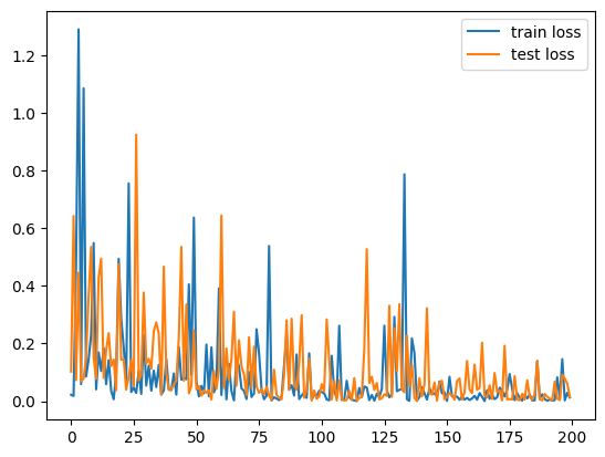
In [35]:
plt.plot(train_loss, label="train loss")
plt.plot(test_loss, label="test loss")
plt.legend()
plt.show()
In [36]:
x_in_reshape = x_in.reshape((-1, 2))
x_in_reshape = torch.from_numpy(x_in_reshape).float()
x_in_reshape = x_in_reshape.to(device)
x_out_pred = net(x_in_reshape)
x_out_pred = x_out_pred.cpu().detach().numpy()
x_out_pred = x_out_pred.reshape(x_in.shape)
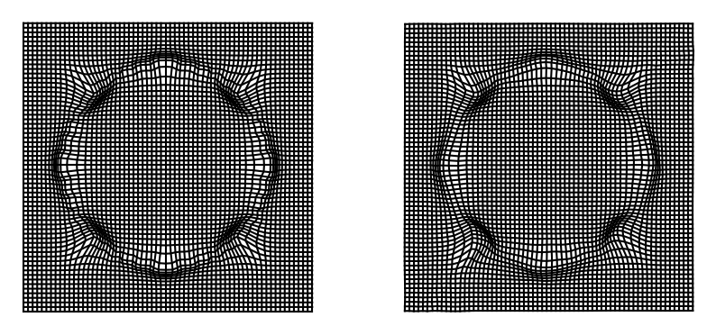
In [37]:
fig = plt.figure(figsize=(10, 10))
ax_in = fig.add_subplot(121)
ax_in = plot_warpgrid(x_out, interval=1)
ax_out = fig.add_subplot(122)
ax_out = plot_warpgrid(x_out_pred, interval=1)
In [22]:
torch.save(net.state_dict(), "model.pt")
In [21]:
res_net = FCNET(
input_dim=2, output_dim=2, n_layers=3, n_neurons=100, activation=torch.nn.Tanh()
)
res_net = res_net.float()
res_state_dict = torch.load("model.pt")
for key in res_state_dict.keys():
res_state_dict[key] = res_state_dict[key].float()
res_net.load_state_dict(res_state_dict)
res_net.to(device)
res_net.eval()
Out [21]:
FCNET(
(layers): ModuleList(
(0): Linear(in_features=2, out_features=100, bias=True)
(1-2): 2 x Linear(in_features=100, out_features=100, bias=True)
(3): Linear(in_features=100, out_features=2, bias=True)
)
(activation): Tanh()
(out): Linear(in_features=100, out_features=2, bias=True)
)
In [33]:
!pip install -q git+https://github.com/johnmarktaylor91/torchlens
In [ ]:
import torchlens as tl
# a little helper function to tell us where our model is
def get_model_device(model):
return next(model.parameters()).device
x = next(iter(dataloaders["train"]))[0][:3] # a sample of our batched training inputs
x = x.to(get_model_device(model))
model_history = tl.log_forward_pass(model, x, vis_opt="unrolled")
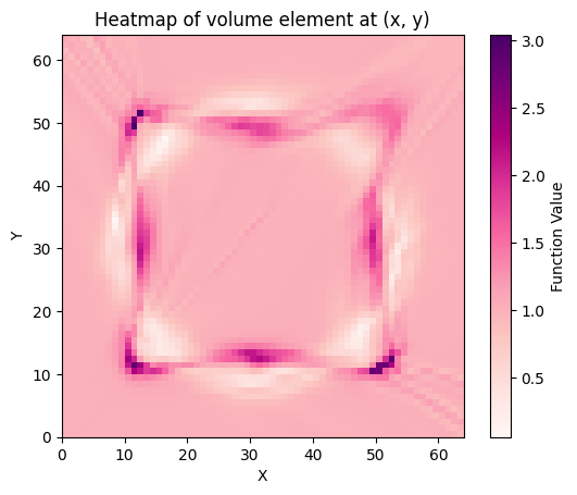
Compute pullback metric#
In [38]:
def get_learned_diffeo(model):
def diffeo(x):
# x = x.to(device)
x = x.float().to(device)
y = model(x)
return y
return diffeo
In [39]:
diffeo = get_learned_diffeo(res_net)
pullback_metric = PullbackMetric(dim=2, embedding_dim=2, immersion=diffeo)
In [40]:
x = gs.linspace(0, 64, 64)
y = gs.linspace(0, 64, 64)
x_grid, y_grid = gs.meshgrid(x, y)
# Combine and reshape the x and y coordinates into a list of 2D points
points = gs.vstack((x_grid.ravel(), y_grid.ravel())).T
# Define your function
def volume_element(x, y):
point = gs.array([x, y])
g = pullback_metric.metric_matrix(point)
vol = gs.sqrt(gs.abs(gs.linalg.det(g)))
return vol
# Apply the function to each point in the list
values = gs.array([volume_element(x, y) for x, y in points])
# Reshape the values back into a 2D grid
z_values = values.reshape(x_grid.shape)
# Create the heatmap
plt.imshow(
z_values, origin="lower", extent=[x.min(), x.max(), y.min(), y.max()], cmap="RdPu"
)
plt.colorbar(label="Function Value")
plt.xlabel("X")
plt.ylabel("Y")
plt.title("Heatmap of volume element at (x, y)")
plt.show()
In [ ]: