Notebook source code: notebooks/07_application_rnns_grid_cells.ipynb
Analyze Path-Integrating Recurrent Neural Networks#
Set Up + Imports#
In [1]:
import setup
setup.main()
%load_ext autoreload
%autoreload 2
# %load_ext jupyter_black
import neurometry.datasets.synthetic as synthetic
from neurometry.datasets.load_rnn_grid_cells import plot_rate_map
from neurometry.datasets.rnn_grid_cells.scores import GridScorer
import numpy as np
import matplotlib.pyplot as plt
import os
os.environ["GEOMSTATS_BACKEND"] = "pytorch"
import geomstats.backend as gs
import torch
from tqdm import tqdm
Working directory: /home/facosta/neurometry/neurometry
Directory added to path: /home/facosta/neurometry
Directory added to path: /home/facosta/neurometry/neurometry
2024-05-16 01:17:27.122166: I tensorflow/core/platform/cpu_feature_guard.cc:210] This TensorFlow binary is optimized to use available CPU instructions in performance-critical operations.
To enable the following instructions: AVX2 FMA, in other operations, rebuild TensorFlow with the appropriate compiler flags.
2024-05-16 01:17:27.799932: W tensorflow/compiler/tf2tensorrt/utils/py_utils.cc:38] TF-TRT Warning: Could not find TensorRT
INFO: Note: detected 128 virtual cores but NumExpr set to maximum of 64, check "NUMEXPR_MAX_THREADS" environment variable.
INFO: Note: NumExpr detected 128 cores but "NUMEXPR_MAX_THREADS" not set, so enforcing safe limit of 8.
INFO: NumExpr defaulting to 8 threads.
Single-Agent RNN#
Load activations across training epochs#
In [2]:
import sys
path = os.path.join(os.getcwd(), "datasets/rnn_grid_cells")
sys.path.append(path)
from neurometry.datasets.load_rnn_grid_cells import load_activations
In [35]:
import argparse
import torch
class Config:
save_dir = "models/" # directory to save trained models
n_epochs = 1 # number of training epochs
n_steps = 1 # batches per epoch
batch_size = 1000 # number of trajectories per batch
sequence_length = 20 # number of steps in trajectory
learning_rate = 1e-4 # gradient descent learning rate
Np = 512 # number of place cells
Ng = 4096 # number of grid cells
place_cell_rf = 0.12 # width of place cell center tuning curve (m)
DoG = True # use difference of gaussians tuning curves
surround_scale = 2 # if DoG, ratio of sigma2^2 to sigma1^2
RNN_type = "RNN" # RNN or LSTM
activation = "relu" # recurrent nonlinearity
weight_decay = 1e-6 # strength of weight decay on recurrent weights
periodic = False # trajectories with periodic boundary conditions
box_width = 2.2 # width of training environment
box_height = 2.2 # height of training environment
# device = (
# "cuda" if torch.cuda.is_available() else "cpu"
# ) # device to use for training
device = torch.device("cuda:7")
n_avg = 50 # number of trajectories to average over for rate maps
# If you need to access the configuration as a dictionary
config = Config.__dict__
def create_parser(config):
parser = argparse.ArgumentParser()
for attr, value in config.items():
if not attr.startswith("__"):
parser.add_argument(
f"--{attr}", type=type(value), default=value, help=f"default: {value}"
)
return parser
parser = create_parser(config)
options, unknown = parser.parse_known_args()
In [57]:
from neurometry.datasets.rnn_grid_cells.model import RNN
from neurometry.datasets.rnn_grid_cells.place_cells import PlaceCells
from neurometry.datasets.rnn_grid_cells.scores import GridScorer
from neurometry.datasets.rnn_grid_cells.trajectory_generator import TrajectoryGenerator
from neurometry.datasets.rnn_grid_cells.utils import generate_run_ID
options.run_ID = generate_run_ID(options)
place_cells = PlaceCells(options)
if options.RNN_type == "RNN":
model = RNN(options, place_cells)
elif options.RNN_type == "LSTM":
raise NotImplementedError
print("Creating trajectory generator...")
trajectory_generator = TrajectoryGenerator(options, place_cells)
print("Loading single agent model...")
model_single_agent = model.to(options.device)
file_path = "datasets/rnn_grid_cells/Single agent path integration high res/Seed 0/steps_20_batch_200_RNN_4096_relu_rf_012_DoG_True_periodic_False_lr_00001_weight_decay_1e-06"
epoch = 10
model_name = "final_model.pth" if epoch == "final" else f"epoch_{epoch}.pth"
model_path = os.path.join(file_path, model_name)
saved_model_single_agent = torch.load(model_path)
model_single_agent.load_state_dict(saved_model_single_agent)
Creating trajectory generator...
Loading single agent model...
Out [57]:
<All keys matched successfully>
In [60]:
from neurometry.datasets.rnn_grid_cells.visualize import compute_ratemaps
print("Computing ratemaps and activations...")
Ng = options.Ng
n_avg = options.n_avg
res = 20
(
activations_single_agent,
rate_map_single_agent,
g_single_agent,
positions_single_agent,
) = compute_ratemaps(
model_single_agent,
trajectory_generator,
options,
res=res,
n_avg=50,
Ng=Ng,
all_activations_flag=True,
)
Computing ratemaps and activations...
Processing: 0%| | 0/50 [00:00<?, ?it/s]Processing: 100%|██████████| 50/50 [04:03<00:00, 4.86s/it]
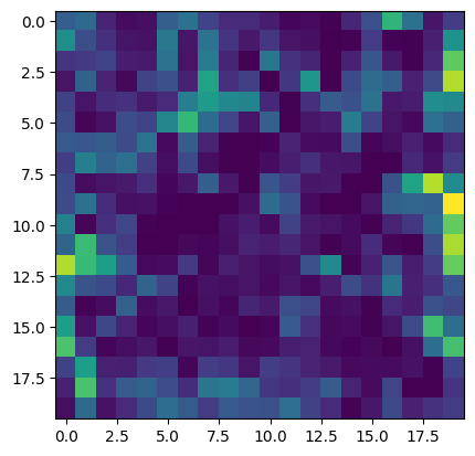
In [56]:
# rm = activations_single_agent.mean(axis=-1)
plt.imshow(rm[0]);
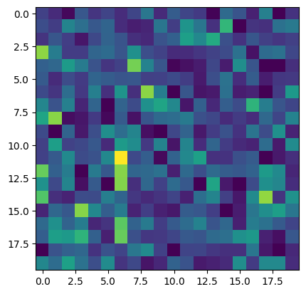
In [63]:
rm_10 = activations_single_agent.mean(axis=-1)
plt.imshow(rm_10[2653]);
In [ ]:
file_path = "datasets/rnn_grid_cells/Single agent path integration high res/Seed 0/steps_20_batch_200_RNN_4096_relu_rf_012_DoG_True_periodic_False_lr_00001_weight_decay_1e-06"
epochs = ["final"]
(activations, rate_maps, state_points) = load_activations(
epochs, file_path, version="single", verbose=True
)
single_agent_positions has shape (batch_size \(\times\) sequence_length \(\times\) n_avg, 2)
In [32]:
box_width = 2.2
res = 20
def downsample_positions(positions, box_width, res):
bin_edges = np.linspace(-box_width / 2, box_width / 2, res + 1)
bin_centers = (bin_edges[:-1] + bin_edges[1:]) / 2
bin_indices_x = np.digitize(positions[:, 0], bins=bin_edges, right=True) - 1
bin_indices_y = np.digitize(positions[:, 1], bins=bin_edges, right=True) - 1
bin_indices_x = np.clip(bin_indices_x, 0, res - 1)
bin_indices_y = np.clip(bin_indices_y, 0, res - 1)
assigned_positions = np.zeros_like(positions)
assigned_positions[:, 0] = bin_centers[bin_indices_x]
assigned_positions[:, 1] = bin_centers[bin_indices_y]
return assigned_positions
new_positions = downsample_positions(single_agent_positions[0], box_width, res)
In [67]:
final_representation = single_agent_rate_maps[0].T
print(final_representation.shape)
box_width = 2.2
res = 20
bin_edges = np.linspace(-box_width / 2, box_width / 2, res + 1)
bin_centers = (bin_edges[:-1] + bin_edges[1:]) / 2
x_centers, y_centers = np.meshgrid(bin_centers, bin_centers[::-1])
positions_array = np.stack([x_centers, y_centers], axis=-1)
# Flatten the coordinate array to shape (400, 2)
positions = positions_array.reshape(-1, 2)
print(positions.shape)
(400, 4096)
(400, 2)
In [4]:
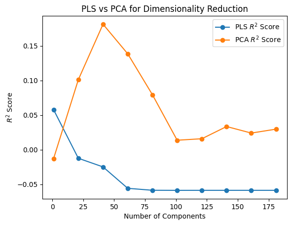
from neurometry.dimension.dimension import evaluate_pls_with_different_K
from neurometry.dimension.dimension import evaluate_PCA_with_different_K
In [73]:
X = final_representation
Y = positions
N = 200
K_values = [i for i in range(1, N + 1, 20)]
pls_r2_scores, pls_transformed_X = evaluate_pls_with_different_K(X, Y, K_values)
pca_r2_scores, pca_transformed_X = evaluate_PCA_with_different_K(X, Y, K_values)
In [74]:
plt.plot(K_values, pls_r2_scores, marker="o", label="PLS $R^2$ Score")
plt.plot(K_values, pca_r2_scores, marker="o", label="PCA $R^2$ Score")
plt.xlabel("Number of Components")
plt.ylabel("$R^2$ Score")
plt.title("PLS vs PCA for Dimensionality Reduction")
plt.legend();
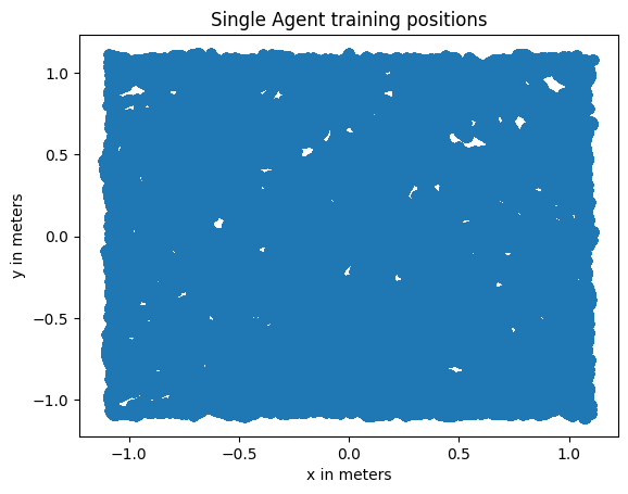
In [20]:
# plot scatter of single_agent_positions
plt.rcParams["text.usetex"] = False
x = single_agent_positions[0][:, 0]
y = single_agent_positions[0][:, 1]
plt.scatter(x, y)
plt.title("Single Agent training positions")
plt.xlabel("x in meters")
plt.ylabel("y in meters");
In [18]:
res = 20
pos = np.zeros((res * res, 2))
print(pos.shape)
(400, 2)
In [88]:
# epochs = list(range(0, 100, 5))
# epochs.append("final")
# file path for 'SA'
sa_file_path = "datasets/rnn_grid_cells/Single agent path integration/Seed 1 weight decay 1e-06/steps_20_batch_200_RNN_4096_relu_rf_012_DoG_True_periodic_False_lr_00001_weight_decay_1e-06"
# file path for 'SA high res'
sa_hr_file_path = "datasets/rnn_grid_cells/Single agent path integration high res/Seed 0/steps_20_batch_200_RNN_4096_relu_rf_012_DoG_True_periodic_False_lr_00001_weight_decay_1e-06"
# file_path for 'DA'
da_file_path = "datasets/rnn_grid_cells/Dual agent path integration disjoint PCs/Seed 1 weight decay 1e-06/steps_20_batch_200_RNN_4096_relu_rf_012_DoG_True_periodic_False_lr_00001_weight_decay_1e-06"
# file_path for 'DA high res'
da_hr_file_path = "datasets/rnn_grid_cells/Dual agent path integration high res/Seed 0/steps_20_batch_200_RNN_4096_relu_rf_012_DoG_True_periodic_False_lr_00001_weight_decay_1e-06"
file_path = da_hr_file_path
epochs = ["final"]
(
single_agent_activations,
single_agent_rate_maps,
single_agent_state_points,
) = load_activations(epochs, file_path, version="dual", verbose=True)
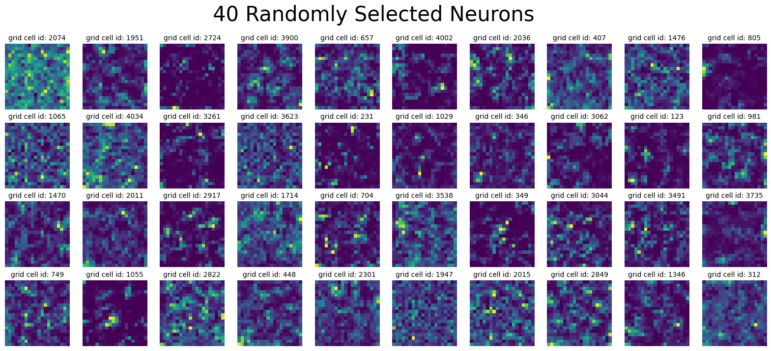
plot_rate_map(
None, 40, single_agent_activations[-1], title="40 Randomly Selected Neurons"
)
Epoch final found.
Loaded epochs ['final'] of dual agent model.
activations has shape (4096, 20, 20, 5). There are 4096 grid cells with 20 x 20 environment resolution, averaged over 5 trajectories.
state_points has shape (4096, 2000). There are 2000 data points in the 4096-dimensional state space.
rate_maps has shape (4096, 400). There are 400 data points averaged over 5 trajectories in the 4096-dimensional state space.
Plot final activations#
In [80]:
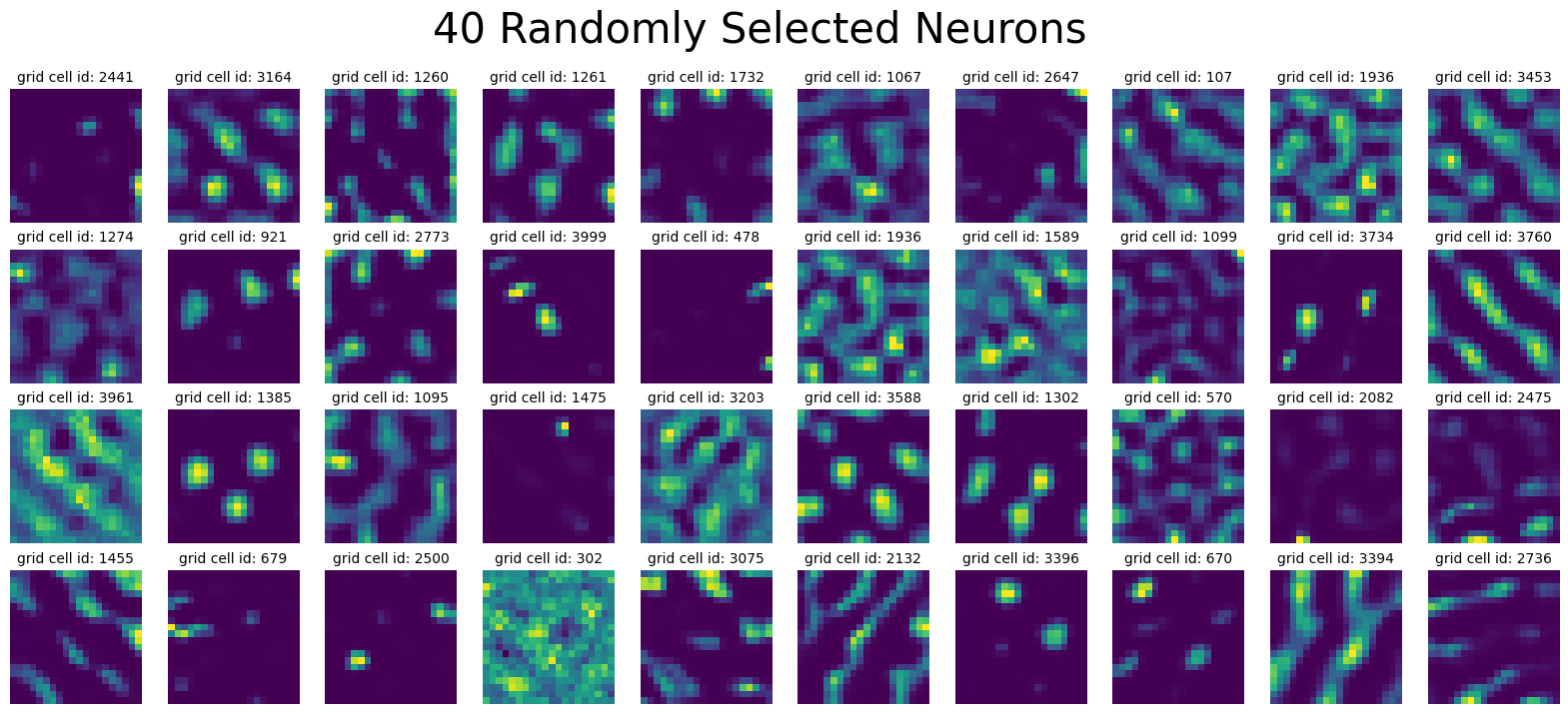
plot_rate_map(
None, 40, single_agent_activations[-1], title="40 Randomly Selected Neurons"
)
Load Training Loss#
In [43]:
model_folder = "Single agent path integration/Seed 1 weight decay 1e-06/"
model_parameters = "steps_20_batch_200_RNN_4096_relu_rf_012_DoG_True_periodic_False_lr_00001_weight_decay_1e-06/"
loss_path = (
"/scratch/facosta/rnn_grid_cells/" + model_folder + model_parameters + "loss.npy"
)
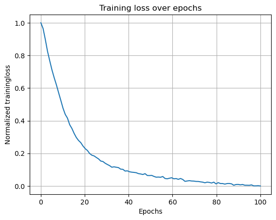
loss = np.load(loss_path)
loss_aggregated = np.mean(loss.reshape(-1, 1000), axis=1)
loss_normalized = (loss_aggregated - np.min(loss_aggregated)) / (
np.max(loss_aggregated) - np.min(loss_aggregated)
)
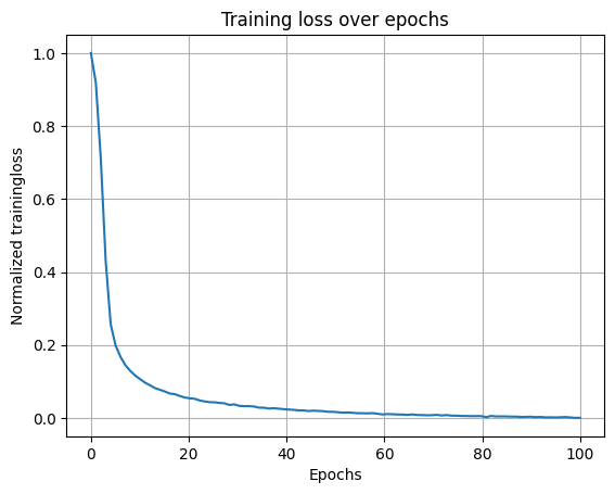
plt.plot(np.linspace(0, 100, 100), loss_normalized)
plt.xlabel("Epochs")
plt.ylabel("Normalized trainingloss")
plt.title("Training loss over epochs")
plt.grid()
Extract representations from epoch = 0 to epoch = 100 (final)#
In [16]:
representations = []
for rep in single_agent_rate_maps:
points = rep.T
norm_points = points / np.linalg.norm(points, axis=1)[:, None]
representations.append(norm_points)
In [17]:
print(
f"There are {representations[0].shape[0]} points in {representations[0].shape[1]}-dimensional space"
)
There are 400 points in 4096-dimensional space
Compute Persistent Homology using \(\texttt{giotto-tda}\)#
In [52]:
from gtda.homology import WeakAlphaPersistence, VietorisRipsPersistence
from gtda.diagrams import PairwiseDistance
from gtda.plotting import plot_diagram, plot_heatmap
import neurometry.datasets.synthetic as synthetic
---------------------------------------------------------------------------
ModuleNotFoundError Traceback (most recent call last)
Cell In[52], line 1
----> 1 from gtda.homology import WeakAlphaPersistence, VietorisRipsPersistence
2 from gtda.diagrams import PairwiseDistance
3 from gtda.plotting import plot_diagram, plot_heatmap
ModuleNotFoundError: No module named 'gtda'
Load synthetic 1-sphere, 2-sphere, and 2-torus neural manifolds
In [20]:
num_points = representations[0].shape[0]
embedding_dim = representations[0].shape[1]
task_points_circle = synthetic.hypersphere(intrinsic_dim=1, num_points=num_points)
_, circle_points = synthetic.synthetic_neural_manifold(
points=task_points_circle,
encoding_dim=embedding_dim,
nonlinearity="linear",
)
norm_circle_points = circle_points / np.linalg.norm(circle_points, axis=1)[:, None]
task_points_sphere = synthetic.hypersphere(intrinsic_dim=2, num_points=num_points)
_, sphere_points = synthetic.synthetic_neural_manifold(
points=task_points_sphere,
encoding_dim=embedding_dim,
nonlinearity="linear",
)
norm_sphere_points = sphere_points / np.linalg.norm(sphere_points, axis=1)[:, None]
task_points_sphere3 = synthetic.hypersphere(intrinsic_dim=3, num_points=num_points)
_, sphere3_points = synthetic.synthetic_neural_manifold(
points=task_points_sphere3,
encoding_dim=embedding_dim,
nonlinearity="linear",
)
norm_sphere3_points = sphere3_points / np.linalg.norm(sphere3_points, axis=1)[:, None]
torus_task_points = synthetic.hypertorus(intrinsic_dim=2, num_points=num_points)
_, torus_points = synthetic.synthetic_neural_manifold(
points=torus_task_points,
encoding_dim=embedding_dim,
nonlinearity="linear",
)
norm_torus_points = torus_points / np.linalg.norm(torus_points, axis=1)[:, None]
torus3_task_points = synthetic.hypertorus(intrinsic_dim=3, num_points=num_points)
_, torus3_points = synthetic.synthetic_neural_manifold(
points=torus3_task_points,
encoding_dim=embedding_dim,
nonlinearity="linear",
)
norm_torus3_points = torus3_points / np.linalg.norm(torus3_points, axis=1)[:, None]
WARNING! Poisson spikes not generated: mean must be non-negative
WARNING! Poisson spikes not generated: mean must be non-negative
WARNING! Poisson spikes not generated: mean must be non-negative
WARNING! Poisson spikes not generated: mean must be non-negative
WARNING! Poisson spikes not generated: mean must be non-negative
In [12]:
num_points = 100
embedding_dim = 10
task_points_circle = synthetic.hypersphere(intrinsic_dim=1, num_points=num_points)
noisy_circle_points, circle_points = synthetic.synthetic_neural_manifold(
points=task_points_circle,
encoding_dim=embedding_dim,
nonlinearity="tanh",
poisson_multiplier=1,
scales=torch.ones(embedding_dim),
)
print(
f"There are {circle_points.shape[0]} points in {circle_points.shape[1]}-dimensional space"
)
noise level: 7.07%
There are 100 points in 10-dimensional space
In [13]:
num_points = 100
embedding_dim = 10
task_points_sphere2 = synthetic.hypersphere(intrinsic_dim=2, num_points=num_points)
noisy_sphere2_points, sphere2_points = synthetic.synthetic_neural_manifold(
points=task_points_sphere2,
encoding_dim=embedding_dim,
nonlinearity="tanh",
poisson_multiplier=1,
scales=torch.ones(embedding_dim),
)
print(
f"There are {sphere2_points.shape[0]} points in {sphere2_points.shape[1]}-dimensional space"
)
noise level: 7.07%
There are 100 points in 10-dimensional space
In [ ]:
num_points = 100
embedding_dim = 10
task_points_torus2 = synthetic.hypertorus(intrinsic_dim=2, num_points=num_points)
noisy_torus2_points, torus2_points = synthetic.synthetic_neural_manifold(
points=task_points_torus2,
encoding_dim=embedding_dim,
nonlinearity="tanh",
poisson_multiplier=1,
scales=torch.ones(embedding_dim),
)
print(
f"There are {torus2_points.shape[0]} points in {sphere2_points.shape[1]}-dimensional space"
)
Load or Compute Vietoris-Rips persistence diagrams
In [21]:
homology_dimensions = (
0,
1,
2,
3,
)
VR = VietorisRipsPersistence(homology_dimensions=homology_dimensions)
In [22]:
try:
print("Loading Vietoris-Rips persistence diagrams")
vr_diagrams = np.load("datasets/rnn_grid_cells/single_agent_vr_pers_diagrams.npy")
except:
print("Computing Vietoris-Rips persistence diagrams")
vr_diagrams = VR.fit_transform(
representations
+ [norm_circle_points]
+ [norm_sphere_points]
+ [norm_torus_points]
+ [norm_sphere3_points]
+ [norm_torus3_points]
)
np.save("datasets/rnn_grid_cells/single_agent_vr_pers_diagrams.npy", vr_diagrams)
print(
f"There are {vr_diagrams.shape[0]} persistence diagrams. Each diagram has {vr_diagrams.shape[1]} features (points)."
)
Loading Vietoris-Rips persistence diagrams
There are 25 persistence diagrams. Each diagram has 1635 features (points).
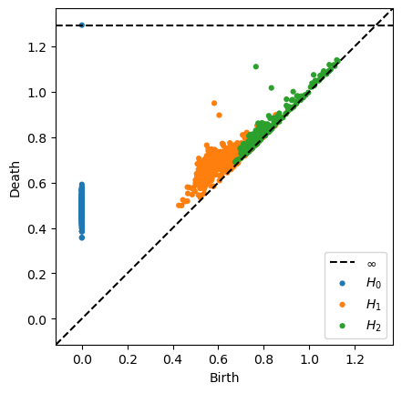
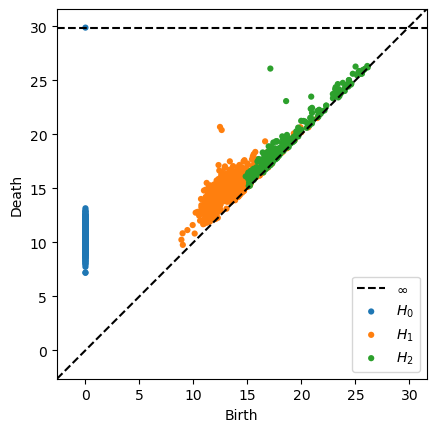
Each feature is a triple \([b, d, q]\), where \(q\) is the dimension, \(b\) is the birth time, \(d\) is the death time
In [23]:
fig_torus3 = plot_diagram(
vr_diagrams[-1],
plotly_params={"title": "Vietoris-Rips Persistence Diagram, 3-torus"},
)
fig_torus3.update_layout(title="Vietoris-Rips Persistence Diagram, 3-torus")
Note: the Poincaré polynomial of a surface is the generating function of its Betti numbers.
the Poincaré polynomial of an \(n\)-torus is \((1+x)^n\), by the Künneth theorem. The Betti numbers are therefore the binomial coefficients.
Thus for the \(3\)-torus, the non-zero Betti numbers are \((1,3,3,1)\).
In [13]:
fig_sphere3 = plot_diagram(
vr_diagrams[-2],
plotly_params={"title": "Vietoris-Rips Persistence Diagram, 3-sphere"},
)
fig_sphere3.update_layout(title="Vietoris-Rips Persistence Diagram, 3-sphere")
In [14]:
fig_rep_final = plot_diagram(
vr_diagrams[-6],
plotly_params={"title": "Vietoris-Rips Persistence Diagram, final representation"},
)
fig_rep_final.update_layout(
title="Vietoris-Rips Persistence Diagram, final representation"
)
Compute pairwise topological distance (“landscape”)#
In [15]:
landscape_PD = PairwiseDistance(metric="landscape", n_jobs=-1)
landscape_distance = landscape_PD.fit_transform(vr_diagrams)
In [20]:
landscape_distance_to_circle = landscape_distance[-5, :-5]
landscape_distance_to_sphere = landscape_distance[-4, :-5]
landscape_distance_to_torus = landscape_distance[-3, :-5]
landscape_distance_to_sphere3 = landscape_distance[-2, :-5]
landscape_distance_to_torus3 = landscape_distance[-1, :-5]
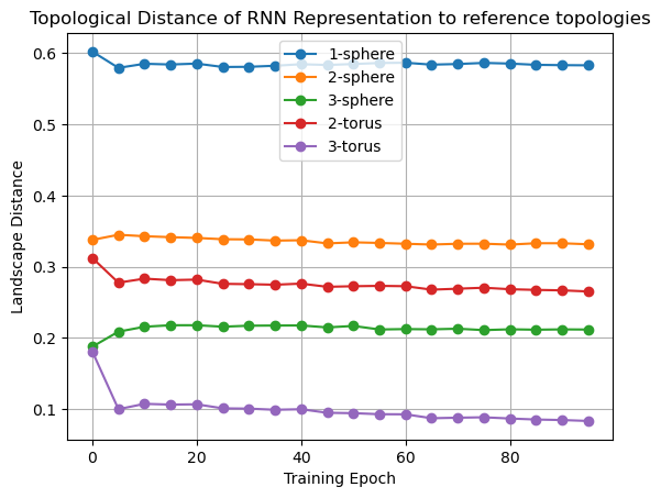
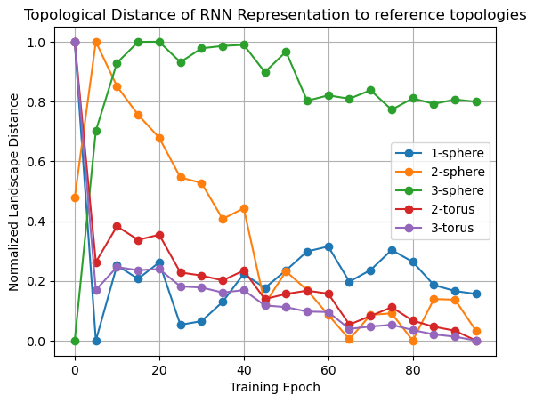
plt.plot(epochs[:-1], landscape_distance_to_circle, "o-", label="1-sphere")
plt.plot(epochs[:-1], landscape_distance_to_sphere, "o-", label="2-sphere")
plt.plot(epochs[:-1], landscape_distance_to_sphere3, "o-", label="3-sphere")
plt.plot(epochs[:-1], landscape_distance_to_torus, "o-", label="2-torus")
plt.plot(epochs[:-1], landscape_distance_to_torus3, "o-", label="3-torus")
plt.xlabel("Training Epoch")
plt.ylabel("Landscape Distance")
plt.title("Topological Distance of RNN Representation to reference topologies")
plt.grid()
plt.legend();
In [19]:
norm_landscape_distance_to_circle = (
landscape_distance_to_circle - np.min(landscape_distance_to_circle)
) / (np.max(landscape_distance_to_circle) - np.min(landscape_distance_to_circle))
norm_landscape_distance_to_sphere = (
landscape_distance_to_sphere - np.min(landscape_distance_to_sphere)
) / (np.max(landscape_distance_to_sphere) - np.min(landscape_distance_to_sphere))
norm_landscape_distance_to_sphere3 = (
landscape_distance_to_sphere3 - np.min(landscape_distance_to_sphere3)
) / (np.max(landscape_distance_to_sphere3) - np.min(landscape_distance_to_sphere3))
norm_landscape_distance_to_torus = (
landscape_distance_to_torus - np.min(landscape_distance_to_torus)
) / (np.max(landscape_distance_to_torus) - np.min(landscape_distance_to_torus))
norm_landscape_distance_to_torus3 = (
landscape_distance_to_torus3 - np.min(landscape_distance_to_torus3)
) / (np.max(landscape_distance_to_torus3) - np.min(landscape_distance_to_torus3))
plt.plot(epochs, norm_landscape_distance_to_circle, "o-", label="1-sphere")
plt.plot(epochs, norm_landscape_distance_to_sphere, "o-", label="2-sphere")
plt.plot(epochs, norm_landscape_distance_to_sphere3, "o-", label="3-sphere")
plt.plot(epochs, norm_landscape_distance_to_torus, "o-", label="2-torus")
plt.plot(epochs, norm_landscape_distance_to_torus3, "o-", label="3-torus")
plt.xlabel("Training Epoch")
plt.ylabel("Normalized Landscape Distance")
plt.title("Topological Distance of RNN Representation to reference topologies")
plt.grid()
plt.legend();
In [95]:
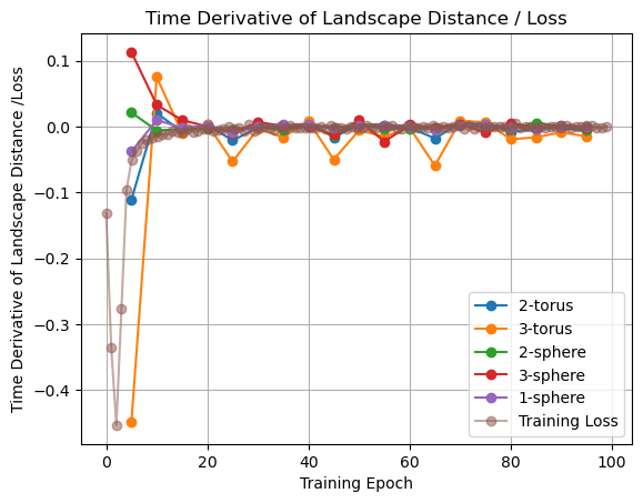
landscape_distance_to_torus_diff = (
np.diff(landscape_distance_to_torus) / landscape_distance_to_torus[:-1]
)
landscape_distance_to_torus3_diff = (
np.diff(landscape_distance_to_torus3) / landscape_distance_to_torus3[:-1]
)
landscape_distance_to_sphere_diff = (
np.diff(landscape_distance_to_sphere) / landscape_distance_to_sphere[:-1]
)
landscape_distance_to_sphere3_diff = (
np.diff(landscape_distance_to_sphere3) / landscape_distance_to_sphere3[:-1]
)
landscape_distance_to_circle_diff = (
np.diff(landscape_distance_to_circle) / landscape_distance_to_circle[:-1]
)
loss_diff = np.diff(loss_normalized) / loss_aggregated[:-1]
plt.plot(epochs[1:], landscape_distance_to_torus_diff, "o-", label="2-torus")
plt.plot(epochs[1:], landscape_distance_to_torus3_diff, "o-", label="3-torus")
plt.plot(epochs[1:], landscape_distance_to_sphere_diff, "o-", label="2-sphere")
plt.plot(epochs[1:], landscape_distance_to_sphere3_diff, "o-", label="3-sphere")
plt.plot(epochs[1:], landscape_distance_to_circle_diff, "o-", label="1-sphere")
plt.plot(np.linspace(0, 99, 99), 10 * loss_diff, "o-", label="Training Loss", alpha=0.5)
plt.xlabel("Training Epoch")
plt.ylabel("Time Derivative of Landscape Distance /Loss")
plt.legend()
plt.title("Time Derivative of Landscape Distance / Loss")
plt.grid();
In [15]:
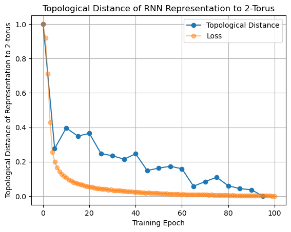
error_normalized = (error - np.min(error)) / (np.max(error) - np.min(error))
loss_normalized = (loss_aggregated - np.min(loss_aggregated)) / (
np.max(loss_aggregated) - np.min(loss_aggregated)
)
In [16]:
plt.plot(epochs, error_normalized, "o-", label="Topological Distance")
plt.plot(np.linspace(0, 100, 100), loss_normalized, "o-", alpha=0.5, label="Loss")
plt.xlabel("Training Epoch")
plt.ylabel("Topological Distance of Representation to 2-torus")
plt.title("Topological Distance of RNN Representation to 2-Torus")
plt.grid()
plt.legend();
In [23]:
fig_epoch_0 = plot_diagram(
vr_diagrams[1],
homology_dimensions=(0, 1, 2),
plotly_params={"title": "Vietoris-Rips PD, single-agent RNN, epoch=0"},
)
fig_epoch_0.update_layout(title="Vietoris-Rips PD, single-agent RNN, epoch=0")
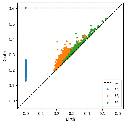
In [24]:
fig_epoch_95 = plot_diagram(
vr_diagrams[-1],
homology_dimensions=(0, 1, 2),
plotly_params={"title": "Vietoris-Rips PD, single-agent RNN, epoch=95"},
)
fig_epoch_95.update_layout(title="Vietoris-Rips PD, single-agent RNN, epoch=95")
In [30]:
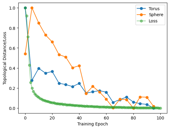
sphere_error_normalized = (sphere_error - np.min(sphere_error)) / (
np.max(sphere_error) - np.min(sphere_error)
)
plt.plot(epochs, error_normalized, "o-", label="Torus")
plt.plot(epochs, sphere_error_normalized, "o-", label="Sphere")
plt.plot(np.linspace(0, 100, 100), loss_normalized, "o-", alpha=0.5, label="Loss")
plt.xlabel("Training Epoch")
plt.ylabel("Topological Distance/Loss")
plt.legend();
Out [30]:
<matplotlib.legend.Legend at 0x7f8f4ad0f0d0>
Estimate rank of connectivity matrix#
Get final model (epoch \(=100\))
Compare run-times of \(\texttt{giotto-tda}, \texttt{ripser}, \texttt{giotto-ph}\)#
In [20]:
from gtda.homology import WeakAlphaPersistence, VietorisRipsPersistence
from ripser import ripser
from persim import plot_diagrams
from gph import ripser_parallel
import time
final_representation = representations[-1]
homology_dimensions = (
0,
1,
2,
)
VR = VietorisRipsPersistence(homology_dimensions=homology_dimensions)
gtda_start = time.time()
gtda_vr_diagrams = VR.fit_transform([final_representation])
gtda_end = time.time()
print(
f"Time to compute Vietoris-Rips persistence diagrams in giotto-tda: {gtda_end - gtda_start:.2f}"
)
ripser_start = time.time()
diagrams = ripser(representations[-1], maxdim=2)["dgms"]
ripser_end = time.time()
print(
f"Time to compute Vietoris-Rips persistence diagrams in ripser: {ripser_end - ripser_start:.2f}"
)
gph_start = time.time()
gph_vr_diagrams = ripser_parallel(final_representation, maxdim=2, n_threads=-1)
gph_end = time.time()
print(
f"Time to compute Vietoris-Rips persistence diagrams in giotto-ph: {gph_end - gph_start:.2f} sec"
)
Time to compute Vietoris-Rips persistence diagrams in giotto-tda: 4.770987272262573
Time to compute Vietoris-Rips persistence diagrams in ripser: 15.016701698303223
Time to compute Vietoris-Rips persistence diagrams in giotto-ph: 3.094177722930908
In [37]:
plot_diagrams(gph_vr_diagrams["dgms"])
In [70]:
diags = ripser_parallel(
representations[-1], maxdim=2, coeff=2, metric="manhattan", n_threads=-1
)["dgms"]
plot_diagrams(diags)
In [71]:
gph_diagrams = {}
for i in range(len(epochs)):
gph_diagrams[epochs[i]] = ripser_parallel(
representations[i], maxdim=2, coeff=2, metric="euclidean", n_threads=-1
)["dgms"]
plot_diagrams(gph_diagrams["final"])
Isolate Grid Cells (cells with high grid score)#
In [18]:
grid_scores_all_epochs = []
band_scores_all_epochs = []
border_scores_all_epochs = []
for epoch in epochs:
scores_dir = (
"/scratch/facosta/rnn_grid_cells/" + model_folder + model_parameters + "scores/"
)
grid_scores_all_epochs.append(
np.load(scores_dir + f"score_60_single_agent_epoch_{epoch}.npy")
)
band_scores_all_epochs.append(
np.load(scores_dir + f"band_scores_single_agent_epoch_{epoch}.npy")
)
border_scores_all_epochs.append(
np.load(scores_dir + f"border_scores_single_agent_epoch_{epoch}.npy")
)
In [19]:
final_epoch_grid_score_sort = np.argsort(grid_scores_all_epochs[-1])
final_epoch_band_score_sort = np.argsort(band_scores_all_epochs[-1])
final_epoch_border_score_sort = np.argsort(border_scores_all_epochs[-1])
sorted_grid_scores_all_epochs = []
sorted_band_scores_all_epochs = []
sorted_border_scores_all_epochs = []
for grid_scores in grid_scores_all_epochs:
sorted_grid_scores_all_epochs.append(grid_scores[final_epoch_grid_score_sort])
for band_scores in band_scores_all_epochs:
sorted_band_scores_all_epochs.append(band_scores[final_epoch_band_score_sort])
for border_scores in border_scores_all_epochs:
sorted_border_scores_all_epochs.append(border_scores[final_epoch_border_score_sort])
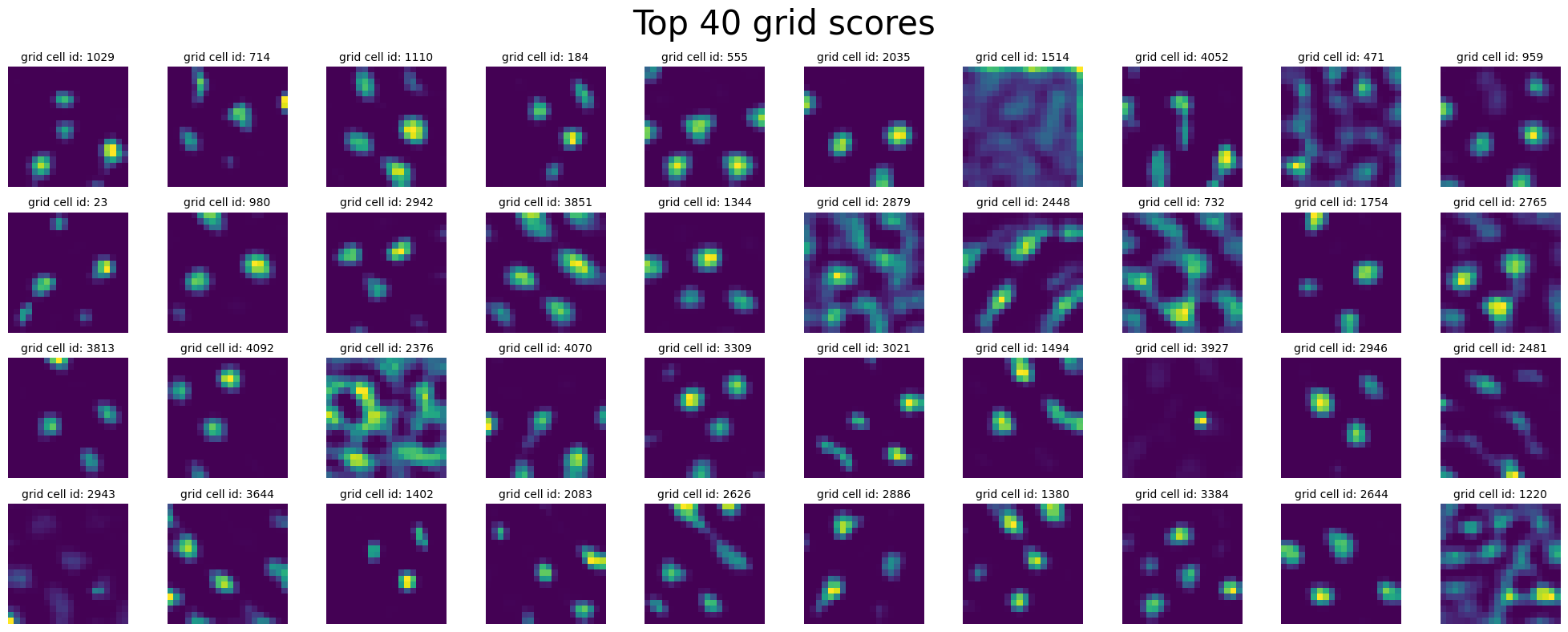
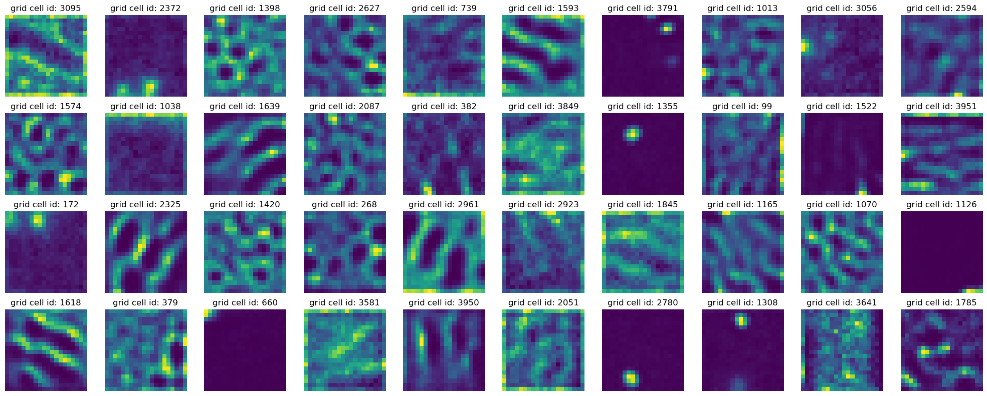
see 40 units with highest grid scores:
In [20]:
plot_rate_map(
final_epoch_grid_score_sort[-40:],
None,
single_agent_activations[-1],
title="Top 40 grid scores",
)
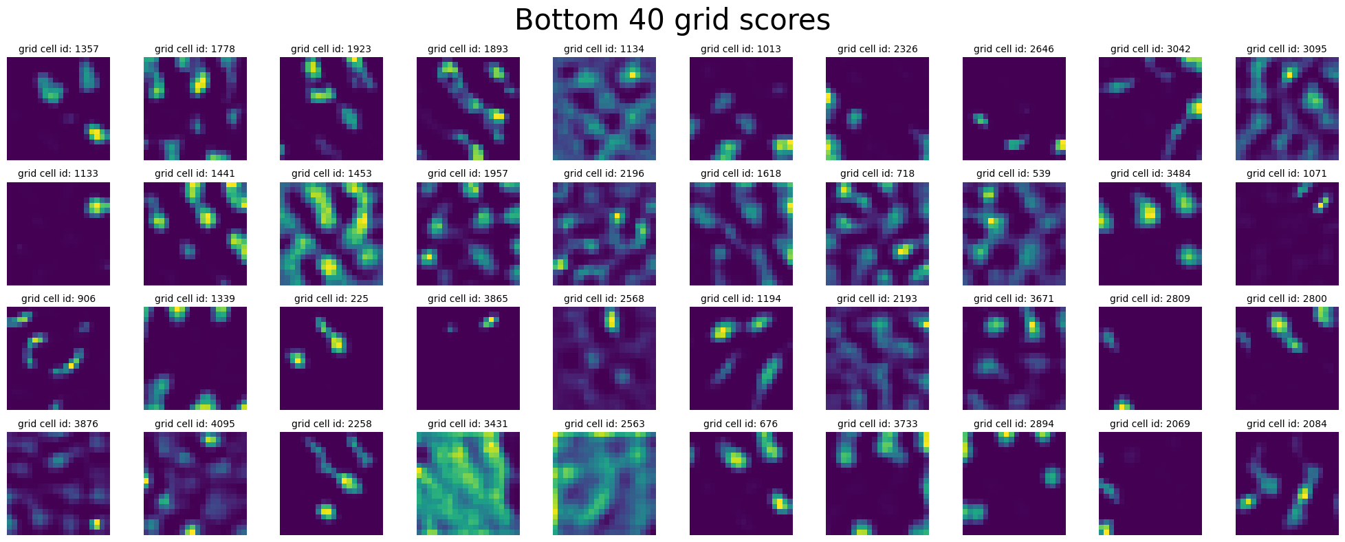
plot_rate_map(
final_epoch_grid_score_sort[:40],
None,
single_agent_activations[-1],
title="Bottom 40 grid scores",
)
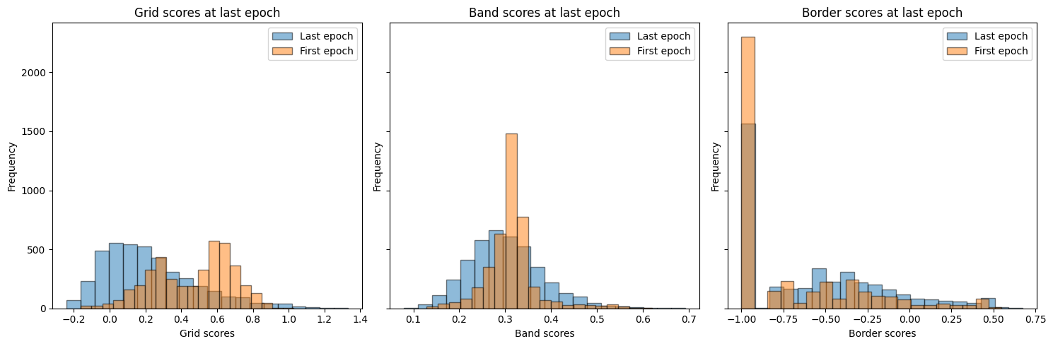
In [21]:
fig, ax = plt.subplots(1, 3, figsize=(15, 5), sharey=True)
ax[0].hist(
grid_scores_all_epochs[-1],
bins=20,
alpha=0.5,
label="Last epoch",
edgecolor="black",
)
ax[0].hist(
grid_scores_all_epochs[0],
bins=20,
alpha=0.5,
label="First epoch",
edgecolor="black",
)
ax[0].set_xlabel("Grid scores")
ax[0].set_ylabel("Frequency")
ax[0].set_title("Grid scores at last epoch")
ax[0].legend()
ax[1].hist(
band_scores_all_epochs[-1],
bins=20,
alpha=0.5,
label="Last epoch",
edgecolor="black",
)
ax[1].hist(
band_scores_all_epochs[0],
bins=20,
alpha=0.5,
label="First epoch",
edgecolor="black",
)
ax[1].set_xlabel("Band scores")
ax[1].set_ylabel("Frequency")
ax[1].set_title("Band scores at last epoch")
ax[1].legend()
ax[2].hist(
border_scores_all_epochs[-1],
bins=20,
alpha=0.5,
label="Last epoch",
edgecolor="black",
)
ax[2].hist(
border_scores_all_epochs[0],
bins=20,
alpha=0.5,
label="First epoch",
edgecolor="black",
)
ax[2].set_xlabel("Border scores")
ax[2].set_ylabel("Frequency")
ax[2].set_title("Border scores at last epoch")
ax[2].legend()
plt.tight_layout()
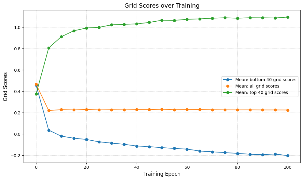
In [22]:
num_top_bottom = 40
lowest_grid_scores_over_time = [
np.mean(sorted_grid_scores_all_epochs[i][:num_top_bottom])
for i in range(len(epochs))
]
top_grid_scores_over_time = [
np.mean(sorted_grid_scores_all_epochs[i][-num_top_bottom:])
for i in range(len(epochs))
]
average_grid_scores_over_time = [
np.mean(sorted_grid_scores_all_epochs[i]) for i in range(len(epochs))
]
In [24]:
fig, ax = plt.subplots(figsize=(10, 6))
ax.plot(
epochs[:-1] + [100],
lowest_grid_scores_over_time,
"o-",
label=f"Mean: bottom {num_top_bottom} grid scores",
)
ax.plot(
epochs[:-1] + [100],
average_grid_scores_over_time,
"o-",
label="Mean: all grid scores",
)
ax.plot(
epochs[:-1] + [100],
top_grid_scores_over_time,
"o-",
label=f"Mean: top {num_top_bottom} grid scores",
)
ax.set_xlabel("Training Epoch", fontsize=12)
ax.set_ylabel("Grid Scores", fontsize=12)
ax.set_title("Grid Scores over Training", fontsize=14)
ax.tick_params(axis="both", which="major", labelsize=10)
ax.grid(True, which="both", linestyle="--", linewidth=0.5, alpha=0.7)
ax.legend()
plt.tight_layout()
plt.show()
In [70]:
selected_indices = final_epoch_band_score_sort[-500:]
r = representations[-1][:, selected_indices]
diagrams = ripser(r, maxdim=2)["dgms"]
plot_diagrams(diagrams)
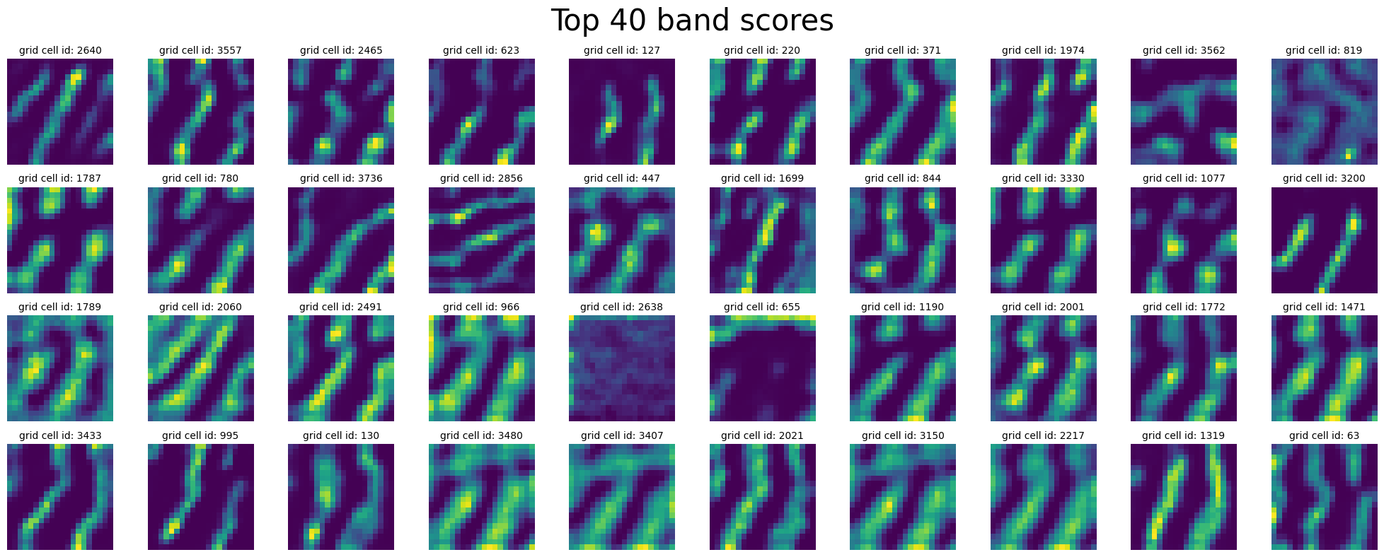
Inspect Band Cells (cells with high band score)#
In [25]:
plot_rate_map(
final_epoch_band_score_sort[-40:],
None,
single_agent_activations[-1],
title="Top 40 band scores",
)
plot_rate_map(
final_epoch_band_score_sort[:40],
None,
single_agent_activations[-1],
title="Bottom 40 band scores",
)
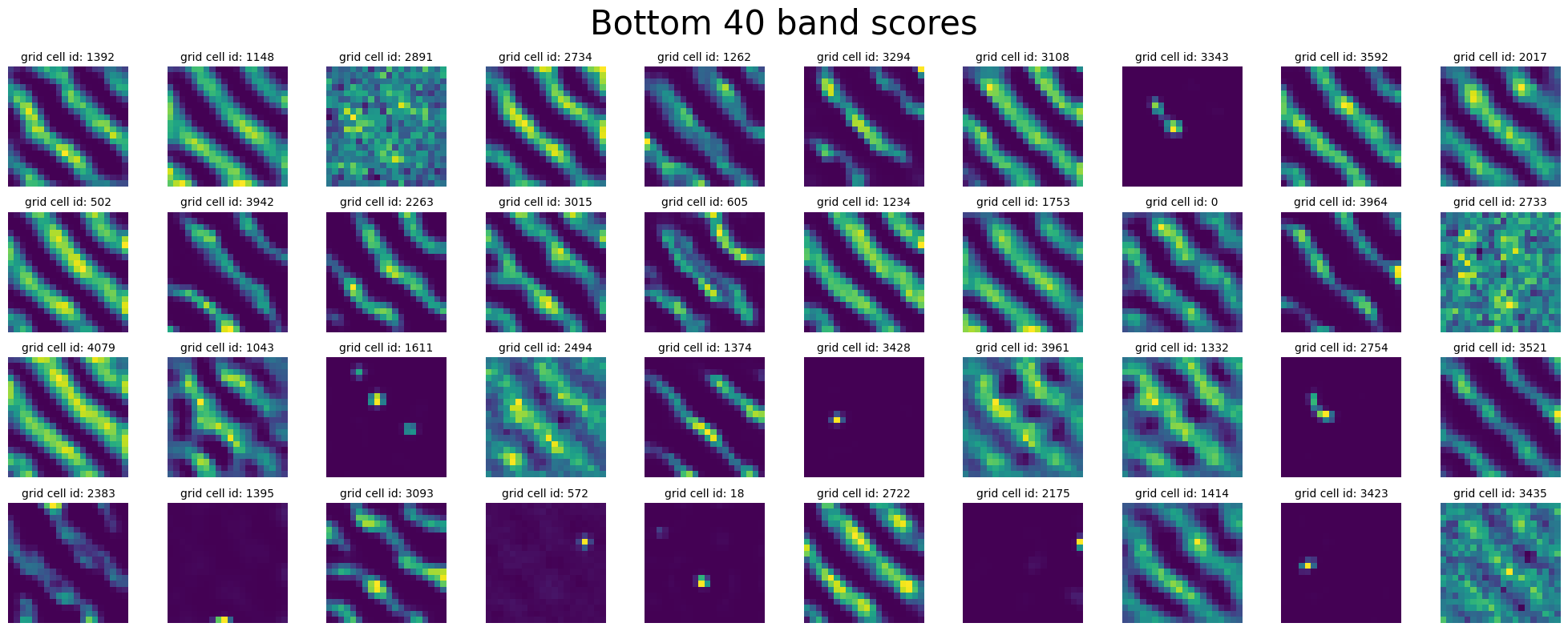
^ why are do these cells have “low” band score ?
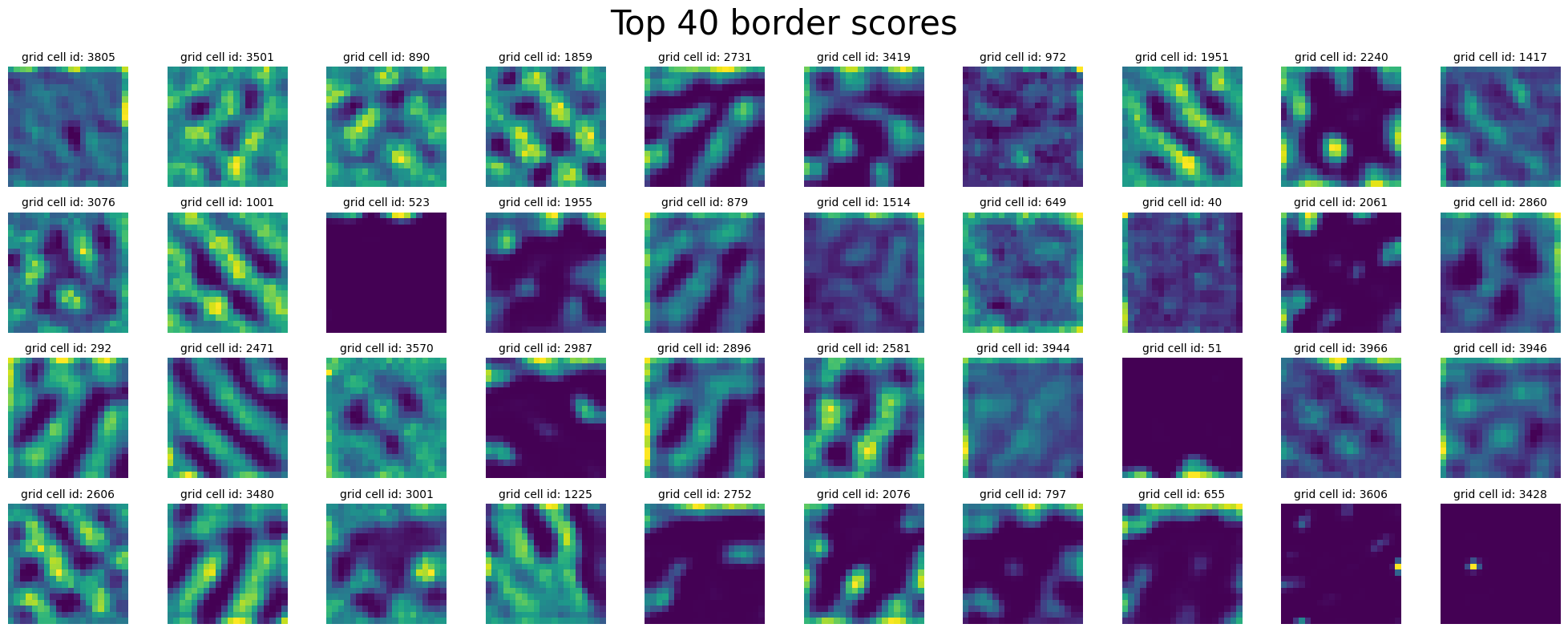
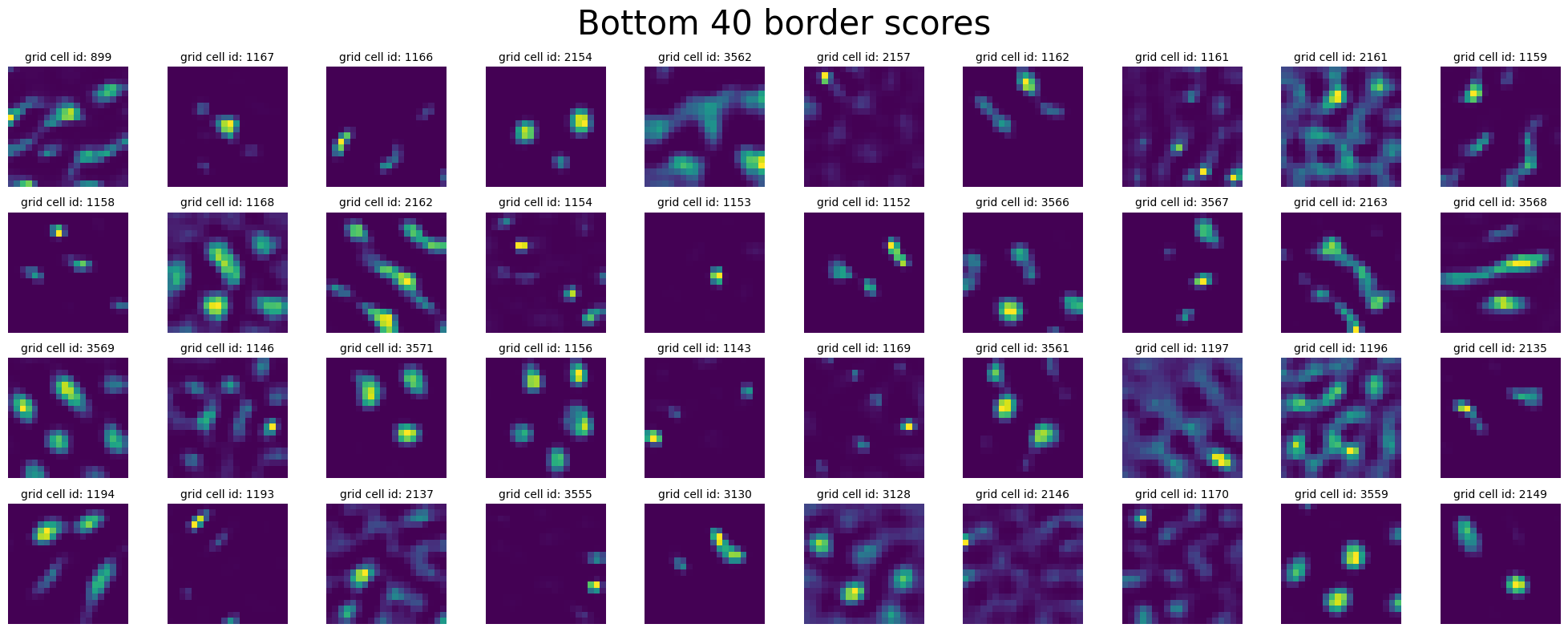
Isolate Border cells (cells with high border score)#
In [26]:
plot_rate_map(
final_epoch_border_score_sort[-40:],
None,
single_agent_activations[-1],
title="Top 40 border scores",
)
plot_rate_map(
final_epoch_border_score_sort[:40],
None,
single_agent_activations[-1],
title="Bottom 40 border scores",
)
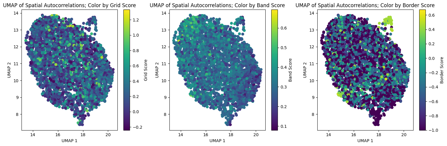
Compute Spatial Autocorrelation + UMAP#
In [27]:
def compute_spatial_autocorrelation(res, rate_map_single_agent, scorer):
print("Computing spatial auto-correlation...")
_, _, _, _, spatial_autocorrelation, _ = zip(
*[scorer.get_scores(rm.reshape(res, res)) for rm in tqdm(rate_map_single_agent)]
)
spatial_autocorrelation = np.array(spatial_autocorrelation)
return spatial_autocorrelation
In [28]:
starts = [0.2] * 10
ends = np.linspace(0.4, 1.0, num=10)
box_width = 2.2
box_height = 2.2
res = 20
coord_range = ((-box_width / 2, box_width / 2), (-box_height / 2, box_height / 2))
masks_parameters = zip(starts, ends.tolist())
scorer = GridScorer(res, coord_range, masks_parameters)
# spatial_autocorrelations = []
# for _, epoch in enumerate(epochs):
spatial_autocorrelation = compute_spatial_autocorrelation(
res, single_agent_rate_maps[-1], scorer
)
print(spatial_autocorrelation.shape)
Computing spatial auto-correlation...
3%|▎ | 143/4096 [00:01<00:30, 128.83it/s]100%|██████████| 4096/4096 [00:31<00:00, 129.28it/s]
(4096, 39, 39)
In [29]:
def z_standardize(matrix):
return (matrix - np.mean(matrix, axis=0)) / np.std(matrix, axis=0)
def vectorized_spatial_autocorrelation_matrix(spatial_autocorrelation):
num_cells = spatial_autocorrelation.shape[0]
num_bins = spatial_autocorrelation.shape[1] * spatial_autocorrelation.shape[2]
spatial_autocorrelation_matrix = np.zeros((num_bins, num_cells))
for i in range(num_cells):
vector = spatial_autocorrelation[i].flatten()
spatial_autocorrelation_matrix[:, i] = vector
return z_standardize(spatial_autocorrelation_matrix)
In [30]:
spatial_autocorrelation_matrix = vectorized_spatial_autocorrelation_matrix(
spatial_autocorrelation
)
print(spatial_autocorrelation_matrix.shape)
(1521, 4096)
In [32]:
import umap
umap_reducer_2d = umap.UMAP(n_components=2, random_state=42)
umap_embedding = umap_reducer_2d.fit_transform(spatial_autocorrelation_matrix.T)
print(umap_embedding.shape)
(4096, 2)
In [37]:
from sklearn.manifold import TSNE
tsne_reducer_2d = TSNE(n_components=2, random_state=42)
tsne_embedding = tsne_reducer_2d.fit_transform(spatial_autocorrelation_matrix.T)
In [33]:
fig, axs = plt.subplots(1, 3, figsize=(15, 5))
# Plot for Grid Scores
sc1 = axs[0].scatter(
umap_embedding[:, 0],
umap_embedding[:, 1],
c=grid_scores_all_epochs[-1],
cmap="viridis",
)
axs[0].set_xlabel("UMAP 1")
axs[0].set_ylabel("UMAP 2")
axs[0].set_title("UMAP of Spatial Autocorrelations; Color by Grid Score")
fig.colorbar(sc1, ax=axs[0], orientation="vertical", label="Grid Score")
# Plot for Band Scores
sc2 = axs[1].scatter(
umap_embedding[:, 0],
umap_embedding[:, 1],
c=band_scores_all_epochs[-1],
cmap="viridis",
)
axs[1].set_xlabel("UMAP 1")
axs[1].set_ylabel("UMAP 2")
axs[1].set_title("UMAP of Spatial Autocorrelations; Color by Band Score")
fig.colorbar(sc2, ax=axs[1], orientation="vertical", label="Band Score")
# Plot for Border Scores
sc3 = axs[2].scatter(
umap_embedding[:, 0],
umap_embedding[:, 1],
c=border_scores_all_epochs[-1],
cmap="viridis",
)
axs[2].set_xlabel("UMAP 1")
axs[2].set_ylabel("UMAP 2")
axs[2].set_title("UMAP of Spatial Autocorrelations; Color by Border Score")
fig.colorbar(sc3, ax=axs[2], orientation="vertical", label="Border Score")
plt.tight_layout()
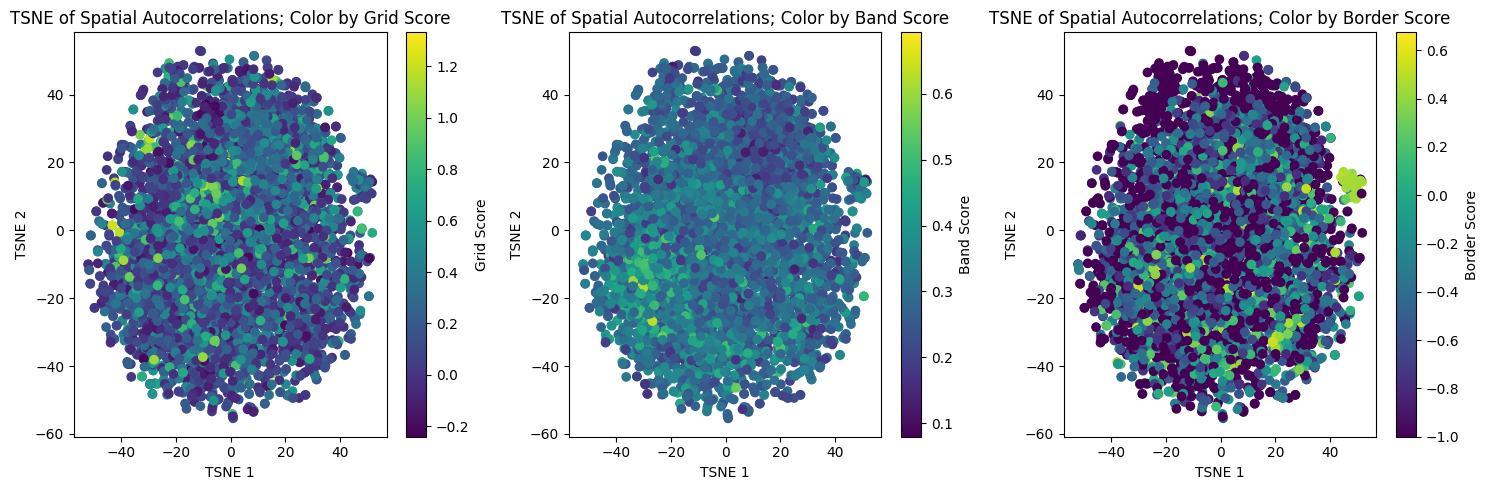
In [38]:
fig, axs = plt.subplots(1, 3, figsize=(15, 5))
# Plot for Grid Scores
sc1 = axs[0].scatter(
tsne_embedding[:, 0],
tsne_embedding[:, 1],
c=grid_scores_all_epochs[-1],
cmap="viridis",
)
axs[0].set_xlabel("TSNE 1")
axs[0].set_ylabel("TSNE 2")
axs[0].set_title("TSNE of Spatial Autocorrelations; Color by Grid Score")
fig.colorbar(sc1, ax=axs[0], orientation="vertical", label="Grid Score")
# Plot for Band Scores
sc2 = axs[1].scatter(
tsne_embedding[:, 0],
tsne_embedding[:, 1],
c=band_scores_all_epochs[-1],
cmap="viridis",
)
axs[1].set_xlabel("TSNE 1")
axs[1].set_ylabel("TSNE 2")
axs[1].set_title("TSNE of Spatial Autocorrelations; Color by Band Score")
fig.colorbar(sc2, ax=axs[1], orientation="vertical", label="Band Score")
# Plot for Border Scores
sc3 = axs[2].scatter(
tsne_embedding[:, 0],
tsne_embedding[:, 1],
c=border_scores_all_epochs[-1],
cmap="viridis",
)
axs[2].set_xlabel("TSNE 1")
axs[2].set_ylabel("TSNE 2")
axs[2].set_title("TSNE of Spatial Autocorrelations; Color by Border Score")
fig.colorbar(sc3, ax=axs[2], orientation="vertical", label="Border Score")
plt.tight_layout()
In [ ]:
In [71]:
reducer_3d = umap.UMAP(n_components=3, random_state=42)
embedding_3d = reducer_3d.fit_transform(spatial_autocorrelation_matrix.T)
print(embedding_3d.shape)
(4096, 2)
In [72]:
import plotly.graph_objects as go
fig = go.Figure(
data=[
go.Scatter3d(
x=embedding_3d[:, 0],
y=embedding_3d[:, 1],
z=embedding_3d[:, 2],
mode="markers",
marker=dict(
size=5,
color=grid_scores_all_epochs[-1],
colorscale="Viridis",
opacity=0.8,
colorbar=dict(title="Grid Score"),
),
)
]
)
fig.update_layout(
title="3D UMAP Visualization of Spatial Autocorrelations; Color by Grid Score",
scene=dict(xaxis_title="UMAP 1", yaxis_title="UMAP 2", zaxis_title="UMAP 3"),
margin=dict(l=0, r=0, b=0, t=30),
)
fig.show()
In [73]:
fig = go.Figure(
data=[
go.Scatter3d(
x=embedding_3d[:, 0],
y=embedding_3d[:, 1],
z=embedding_3d[:, 2],
mode="markers",
marker=dict(
size=5,
color=band_scores_all_epochs[-1],
colorscale="Viridis",
opacity=0.8,
colorbar=dict(title="Band Score"),
),
)
]
)
fig.update_layout(
title="3D UMAP Visualization of Spatial Autocorrelations; Color by Band Score",
scene=dict(xaxis_title="UMAP 1", yaxis_title="UMAP 2", zaxis_title="UMAP 3"),
margin=dict(l=0, r=0, b=0, t=30),
)
fig.show()
In [74]:
fig = go.Figure(
data=[
go.Scatter3d(
x=embedding_3d[:, 0],
y=embedding_3d[:, 1],
z=embedding_3d[:, 2],
mode="markers",
marker=dict(
size=5,
color=border_scores_all_epochs[-1],
colorscale="Viridis",
opacity=0.8,
colorbar=dict(title="Border Score"),
),
)
]
)
fig.update_layout(
title="3D UMAP Visualization of Spatial Autocorrelations; Color by Border Score",
scene=dict(xaxis_title="UMAP 1", yaxis_title="UMAP 2", zaxis_title="UMAP 3"),
margin=dict(l=0, r=0, b=0, t=30),
)
fig.show()
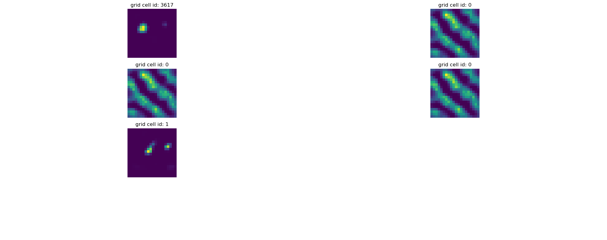
In [29]:
from neurometry.datasets.load_rnn_grid_cells import plot_rate_map
plot_rate_map([3617, 0, 0, 0, 1], 40, single_agent_activations[-1])
Discover “modules” through clustering / dim reduction? (see Gardner Extended Data Fig. 2)#
In [26]:
# parent_dir = os.getcwd() + "/datasets/rnn_grid_cells/"
parent_dir = "/scratch/facosta/rnn_grid_cells/"
single_model_folder = "Single agent path integration/Seed 1 weight decay 1e-06/"
single_model_parameters = "steps_20_batch_200_RNN_4096_relu_rf_012_DoG_True_periodic_False_lr_00001_weight_decay_1e-06/"
saved_model_single_agent = torch.load(
parent_dir + single_model_folder + single_model_parameters + "final_model.pth"
)
print(f"The model is a dictionary with keys {saved_model_single_agent.keys()}")
The model is a dictionary with keys odict_keys(['encoder.weight', 'RNN.weight_ih_l0', 'RNN.weight_hh_l0', 'decoder.weight'])
Extract the recurrent connectivity matrix:
In [27]:
W = saved_model_single_agent["RNN.weight_hh_l0"].detach().numpy()
print(f"W has dimensions {W.shape}")
W has dimensions (4096, 4096)
Find singular values of \(W\):
In [33]:
singular_values = np.linalg.svd(W, compute_uv=False)
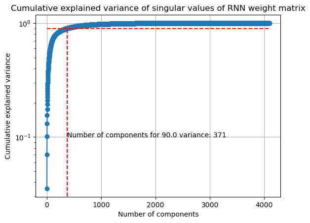
Plot singular value spectrum:
In [57]:
ev_threshold = 0.9
explained_variance = singular_values**2 / np.sum(singular_values**2)
cumulative_explained_variance = np.cumsum(explained_variance)
plt.plot(cumulative_explained_variance, "o-")
plt.xlabel("Number of components")
plt.ylabel("Cumulative explained variance")
plt.yscale("log")
plt.grid()
plt.title("Cumulative explained variance of singular values of RNN weight matrix")
plt.hlines(
ev_threshold, 0, len(cumulative_explained_variance), linestyles="dashed", colors="r"
)
plt.vlines(
np.where(cumulative_explained_variance >= ev_threshold)[0][0],
0,
ev_threshold,
linestyles="dashed",
colors="r",
)
# show number of components to explain 90% of variance on x-axis
plt.text(
np.where(cumulative_explained_variance >= ev_threshold)[0][0],
0.1,
f"Number of components for {100*ev_threshold} variance: {np.where(cumulative_explained_variance >= ev_threshold)[0][0]}",
)
num_components = np.where(cumulative_explained_variance >= ev_threshold)[0][0] + 1
print(
f"Number of components to explain {100*ev_threshold}% of variance: {num_components}"
)
Number of components to explain 90.0% of variance: 372
Dual-Agent RNN#
Load activations across training epochs#
In [97]:
epochs = list(range(0, 100, 5))
(
dual_agent_activations,
dual_agent_rate_maps,
dual_agent_state_points,
) = load_activations(epochs, version="dual", verbose=True)
Epoch 0 found!!! :D
Epoch 5 found!!! :D
Epoch 10 found!!! :D
Epoch 15 found!!! :D
Epoch 20 found!!! :D
Epoch 25 found!!! :D
Epoch 30 found!!! :D
Epoch 35 found!!! :D
Epoch 40 found!!! :D
Epoch 45 found!!! :D
Epoch 50 found!!! :D
Epoch 55 found!!! :D
Epoch 60 found!!! :D
Epoch 65 found!!! :D
Epoch 70 found!!! :D
Epoch 75 found!!! :D
Epoch 80 found!!! :D
Epoch 85 found!!! :D
Epoch 90 found!!! :D
Epoch 95 found!!! :D
Loaded epochs [0, 5, 10, 15, 20, 25, 30, 35, 40, 45, 50, 55, 60, 65, 70, 75, 80, 85, 90, 95] of dual agent model.
There are 4096 grid cells with 20 x 20 environment resolution, averaged over 50 trajectories.
There are 20000 data points in the 4096-dimensional state space.
There are 400 data points averaged over 50 trajectories in the 4096-dimensional state space.
Plot final activations#
In [98]:
plot_rate_map(40, dual_agent_activations[-1])
Extract dual agent representations from epoch = 0 to epoch = 95#
In [99]:
dual_representations = []
for rep in dual_agent_rate_maps:
points = rep.T
norm_points = points / np.linalg.norm(points, axis=1)[:, None]
dual_representations.append(norm_points)
Load training loss#
In [103]:
model_folder = "Dual agent path integration disjoint PCs/Seed 1 weight decay 1e-06/"
model_parameters = "steps_20_batch_200_RNN_4096_relu_rf_012_DoG_True_periodic_False_lr_00001_weight_decay_1e-06/"
loss_path = (
os.getcwd()
+ "/datasets/rnn_grid_cells/"
+ model_folder
+ model_parameters
+ "loss.npy"
)
loss = np.load(loss_path)
loss_aggregated = np.mean(loss.reshape(-1, 1000), axis=1)
loss_normalized = (loss_aggregated - np.min(loss_aggregated)) / (
np.max(loss_aggregated) - np.min(loss_aggregated)
)
plt.plot(np.linspace(0, 100, 100), loss_normalized)
plt.xlabel("Epochs")
plt.ylabel("Normalized trainingloss")
plt.title("Training loss over epochs")
plt.grid()
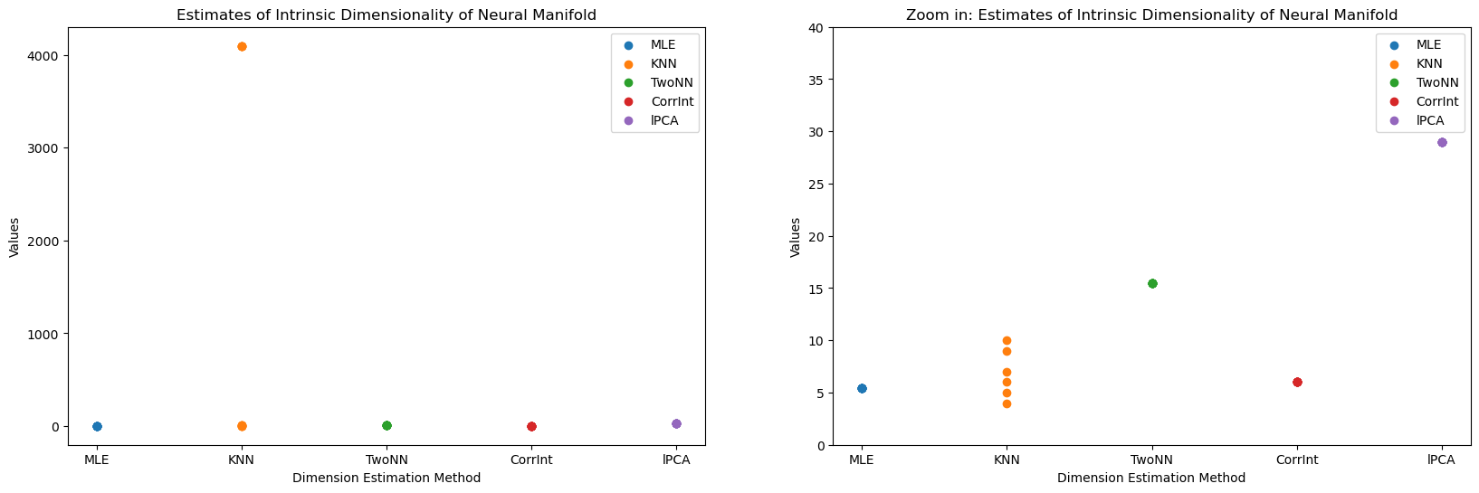
Estimate Dimension#
In [3]:
neural_manifold = rate_maps.T
num_trials = 10
# methods = [method for method in dir(skdim.id) if not method.startswith("_")]
methods = ["MLE", "KNN", "TwoNN", "CorrInt", "lPCA"]
id_estimates = {}
for method_name in methods:
method = getattr(skdim.id, method_name)()
estimates = np.zeros(num_trials)
for trial_idx in range(num_trials):
method.fit(neural_manifold)
estimates[trial_idx] = np.mean(method.dimension_)
id_estimates[method_name] = estimates
In [6]:
neural_manifold.shape
Out [6]:
(400, 4096)
In [18]:
# make side by side plots
fig, axes = plt.subplots(1, 2, figsize=(20, 6))
for i, method in enumerate(methods):
y = id_estimates[method]
x = np.repeat(i, len(y))
axes[0].scatter(x, y, label=method)
axes[1].scatter(x, y, label=method)
axes[0].set_xticks(range(len(methods)))
axes[0].set_xticklabels(methods)
axes[0].set_xlabel("Dimension Estimation Method")
axes[0].set_ylabel("Values")
axes[0].set_title("Estimates of Intrinsic Dimensionality of Neural Manifold")
axes[0].legend()
axes[1].set_xticks(range(len(methods)))
axes[1].set_xticklabels(methods)
axes[1].set_xlabel("Dimension Estimation Method")
axes[1].set_ylabel("Values")
axes[1].set_ylim([0, 40])
axes[1].set_title("Zoom in: Estimates of Intrinsic Dimensionality of Neural Manifold")
axes[1].legend();
estimate extrinsic with PCA, then do nonlinear dim est