Notebook source code: notebooks/06_application_synthetic_v1.ipynb

Synthetic V1: Klein bottle

Lead author: Sofia Gonzalez.

The Klein bottle may be constructed from the symmetry properties of simple cell receptive fields in V1 (See Looking into a Klein bottle by Nicholas V. Swindale). The notion of Klein bottle, written \(\mathbb{K}\), refers to any topological space homeomorphic to that obtained by identification in a full square of the opposite sides with a change of direction for one of the pairs. Group theoretically speaking: :nbsphinx-math:`begin{align*}

& (x_1,y_1) sim (x_2, y_2) \ Leftrightarrow quad & y_1-y_2 in mathbb Z

text{ and } x_1-x_2 in 2mathbb Z \

text{ or } quad &

y_1 + y_2 in mathbb Z text{ and } x_1-x_2 in mathbb Zsetminus 2mathbb Z.

end{align*}`

The intrinsic dimension of the Klein function is 2. This is what geomstats outputs by default when generating random points on its surface. However, we can play with its different parametrizations to work with it in a more intuitive way. It cannot be embedded in \(\mathbb{R}^3\), but only immerged with a self-intersection. The smallest number of dimensions required to embed the Klein bottle is 4. However, we can construct different parametrizations in \(\mathbb{R}^3\) in order to visualize its properties better. The three main 3D parametrizations are: - Klein bottle - Klein bagel - Pinched torus

Set-up + Imports

import setup

setup.main()
%load_ext autoreload
%autoreload 2
%load_ext jupyter_black

import neurometry.datasets.synthetic as synthetic
import numpy as np

import matplotlib.pyplot as plt

import os

os.environ["GEOMSTATS_BACKEND"] = "pytorch"
import geomstats.backend as gs

import plotly.graph_objects as go
from plotly.subplots import make_subplots
import torch

Working directory:  /home/sghomedir/Desktop/github/neurometry/neurometry
Directory added to path:  /home/sghomedir/Desktop/github/neurometry
Directory added to path:  /home/sghomedir/Desktop/github/neurometry/neurometry
The autoreload extension is already loaded. To reload it, use:
  %reload_ext autoreload
The jupyter_black extension is already loaded. To reload it, use:
  %reload_ext jupyter_black

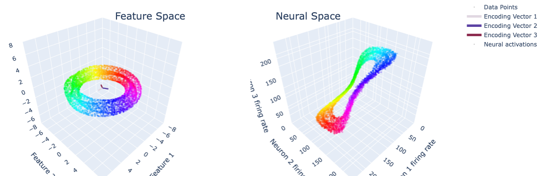
Klein bagel parametrization

num_points = 5000
task_points = synthetic.klein_bottle(num_points, coords_type="bagel")

noisy_points, manifold_points = synthetic.synthetic_neural_manifold(
    points=task_points,
    encoding_dim=3,
    nonlinearity="sigmoid",
    scales=gs.array(np.ones(3)),
    poisson_multiplier=50,
)

print("Initial dimension (task points):", np.shape(task_points)[1])
print("Dimension of manifold/noisy points:", np.shape(noisy_points)[1])

Initial dimension (task points): 3
Dimension of manifold/noisy points: 3

def plot_feature_neural_spaces(
    task_points, noisy_points, range_ax, pt_size=2, opacity=0.5, N=3
):
    x = task_points[:, 0]
    y = task_points[:, 1]
    z = task_points[:, 2]
    angles = torch.atan2(task_points[:, 1], task_points[:, 0])
    normalized_angles = angles / (2 * np.pi) + 1 / 2
    colors = plt.cm.hsv(normalized_angles)

    place_angles = np.linspace(0, 2 * np.pi, N, endpoint=False)
    encoding_matrix = gs.vstack((gs.cos(place_angles), gs.sin(place_angles)))
    vectors = [encoding_matrix[:, i] for i in range(N)]

    cm = plt.get_cmap("twilight")
    vector_colors = [cm(1.0 * i / N) for i in range(N)]
    vector_colors = [
        "rgb({}, {}, {})".format(int(r * 255), int(g * 255), int(b * 255))
        for r, g, b, _ in vector_colors
    ]

    scatter1 = go.Scatter3d(
        x=x,
        y=y,
        z=z,
        mode="markers",
        marker=dict(size=pt_size, color=colors, opacity=opacity),
        name="Data Points",
    )

    lines_and_cones = []
    for idx, (vector, color) in enumerate(zip(vectors, vector_colors)):
        lines_and_cones.append(
            go.Scatter3d(
                x=[0, vector[0]],
                y=[0, vector[1]],
                z=[0, 0],
                mode="lines",
                line=dict(color=color, width=5),
                name=f"Encoding Vector {idx+1}",
            )
        )
    lines_and_cones.append(
        go.Cone(
            x=[vector[0]],
            y=[vector[1]],
            z=[0],
            u=[vector[0] / 10],
            v=[vector[1] / 10],
            w=[0],
            showscale=False,
            colorscale=[[0, color], [1, color]],
            sizemode="absolute",
            sizeref=0.1,
        )
    )

    x = noisy_points[:, 0]
    y = noisy_points[:, 1]
    z = noisy_points[:, 2]

    print(f"mean firing rate: {torch.mean(noisy_points):.2f} Hz")

    scatter2 = go.Scatter3d(
        x=x,
        y=y,
        z=z,
        mode="markers",
        marker=dict(size=pt_size, color=colors, opacity=opacity),
        name="Neural activations",
    )

    fig = make_subplots(
        rows=1, cols=2, specs=[[{"type": "scatter3d"}, {"type": "scatter3d"}]]
    )

    # Add the first set of traces (scatter1 and lines_and_cones) to the first subplot
    fig.add_traces(
        [scatter1] + lines_and_cones,
        rows=[1] * (len([scatter1]) + len(lines_and_cones)),
        cols=[1] * (len([scatter1]) + len(lines_and_cones)),
    )

    # Add the second scatter (scatter2) to the second subplot
    fig.add_trace(scatter2, row=1, col=2)

    reference_frequency = 200

    fig.update_layout(
        scene1=dict(
            aspectmode="cube",
            xaxis=dict(range=[-range_ax, range_ax], title="Feature 1"),
            yaxis=dict(range=[-range_ax, range_ax], title="Feature 2"),
            zaxis=dict(range=[-range_ax, range_ax], title=""),
        ),
        scene2=dict(
            aspectmode="cube",
            xaxis=dict(
                range=[0, reference_frequency * 1.2],
                title="Neuron 1 firing rate",
            ),
            yaxis=dict(
                range=[0, reference_frequency * 1.2],
                title="Neuron 2 firing rate",
            ),
            zaxis=dict(
                range=[0, reference_frequency * 1.2],
                title="Neuron 3 firing rate",
            ),
        ),
        margin=dict(l=0, r=0, b=0, t=0),
        title_text="",
        annotations=[
            dict(
                text="Feature Space",
                xref="paper",
                yref="paper",
                x=0.25,
                y=0.95,
                showarrow=False,
                font=dict(size=20),
            ),
            dict(
                text="Neural Space",
                xref="paper",
                yref="paper",
                x=0.75,
                y=0.95,
                showarrow=False,
                font=dict(size=20),
            ),
        ],
    )

    fig.show()

range_ax = 8
pt_size = 2
opacity = 0.3

plot_feature_neural_spaces(task_points, noisy_points, range_ax, pt_size, opacity)

mean firing rate: 100.24 Hz

Klein bottle parametrization

num_points = 5000
task_points = synthetic.klein_bottle(num_points, coords_type="bottle")
task_points -= gs.mean(task_points)

noisy_points, manifold_points = synthetic.synthetic_neural_manifold(
    points=task_points,
    encoding_dim=3,
    nonlinearity="sigmoid",
    scales=gs.array(np.ones(3)),
    poisson_multiplier=100,
)

print("Initial dimension (task points):", np.shape(task_points)[1])
print("Dimension of manifold/noisy points:", np.shape(noisy_points)[1])

Initial dimension (task points): 3
Dimension of manifold/noisy points: 3

range_ax = 4
pt_size = 2
opacity = 0.3

plot_feature_neural_spaces(task_points, noisy_points, range_ax, pt_size, opacity)

mean firing rate: 109.97 Hz

Data type cannot be displayed: application/vnd.plotly.v1+json